Plotting: Exercises

Note

These exercises are optional.

Previous code

# install.packages("tidyverse")
# install.packages("here")

library(tidyverse)
library(here)

## Load the data
characters <- readRDS(file = here::here("raw_data", "characters.rds"))
psych_stats <- read.csv(
  file = here::here("raw_data", "psych_stats.csv"),
  sep = ";"
)

## Reshape into long format:
psych_stats <- psych_stats %>%
  pivot_longer(
    cols = messy_neat:innocent_jaded,
    names_to = "question",
    values_to = "rating"
  )

## Merge it
characters_stats <- merge(
  x = characters,
  y = psych_stats,
  by.x = "id",
  by.y = "char_id"
)

Exercise 1

Now, let’s make a nice plot out of the data we’ve got.

First of all, let’s clean up our questions column a bit. Replace all “_” characters with “/” characters to make it clearer that we have two poles. Use the internet to figure out which function you need.

Hint

Use gsub(). Look at ?gsub() to see how it works.

Solution

characters_stats$question <- gsub("_", "/", characters_stats$question)

Select up to 40 questions you want to display in the plot and save them into a new vector.

Solution

I’m just gonna take the first 40 questions from all unique ones:

questions <- unique(characters_stats$question)[1:40]
questions

 [1] "messy/neat"                    "disorganized/self.disciplined"
 [3] "diligent/lazy"                 "on.time/tardy"                
 [5] "competitive/cooperative"       "scheduled/spontaneous"        
 [7] "ADHD/OCD"                      "chaotic/orderly"              
 [9] "motivated/unmotivated"         "bossy/meek"                   
[11] "persistent/quitter"            "overachiever/underachiever"   
[13] "muddy/washed"                  "beautiful/ugly"               
[15] "slacker/workaholic"            "driven/unambitious"           
[17] "outlaw/sheriff"                "precise/vague"                
[19] "bad.cook/good.cook"            "manicured/scruffy"            
[21] "lenient/strict"                "relaxed/tense"                
[23] "demanding/unchallenging"       "drop.out/valedictorian"       
[25] "go.getter/slugabed"            "competent/incompetent"        
[27] "aloof/obsessed"                "flexible/rigid"               
[29] "active/slothful"               "loose/tight"                  
[31] "pointed/random"                "fresh/stinky"                 
[33] "dominant/submissive"           "anxious/calm"                 
[35] "clean/perverted"               "neutral/opinionated"          
[37] "always.down/picky"             "hurried/leisurely"            
[39] "attractive/repulsive"          "devoted/unfaithful"

Select one show (your favorite), extract it from the data frame and save it into a new data set. It should only contain the questions you have selected in the first step.

Solution

characters_subset <- characters_stats %>%
  filter(
    uni_name == "Friends",
    question %in% questions
  )

Build the coordinate system of the plot. Plot the rating on the x axis and the question on the y axis.

Solution

p <- ggplot(
  data = characters_subset,
  aes(
    x = rating,
    y = question
  )
)

p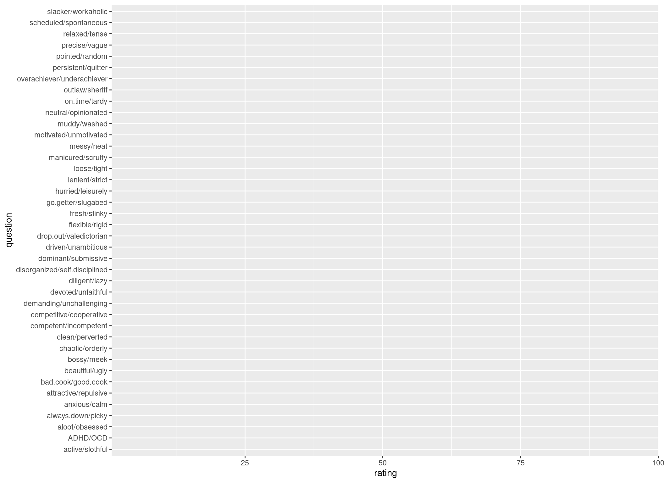

Now let’s split up the plot, so every character gets an own pane. Use facet_grid() to do that.

Hint

Use ?facet_grid to find out how to use it.

Solution

p <- p +
  facet_grid(. ~ name)
p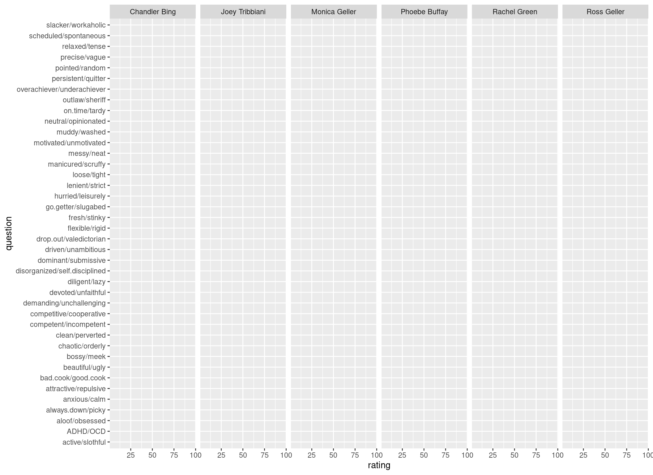

Let’s add bars to the plot by using geom_col(). The filling of the bars should depend on the rating. You might also want to change the width of the bars to fit everything on the page.

Hint

You can change a lot in the appearance of the bars. For example, you might want to use width to make the bars a bit smaller. Or use color to give them a frame.

Solution

p <- p +
  geom_col(
    aes(fill = rating),
    colour = "black",
    width = 0.5
  )

p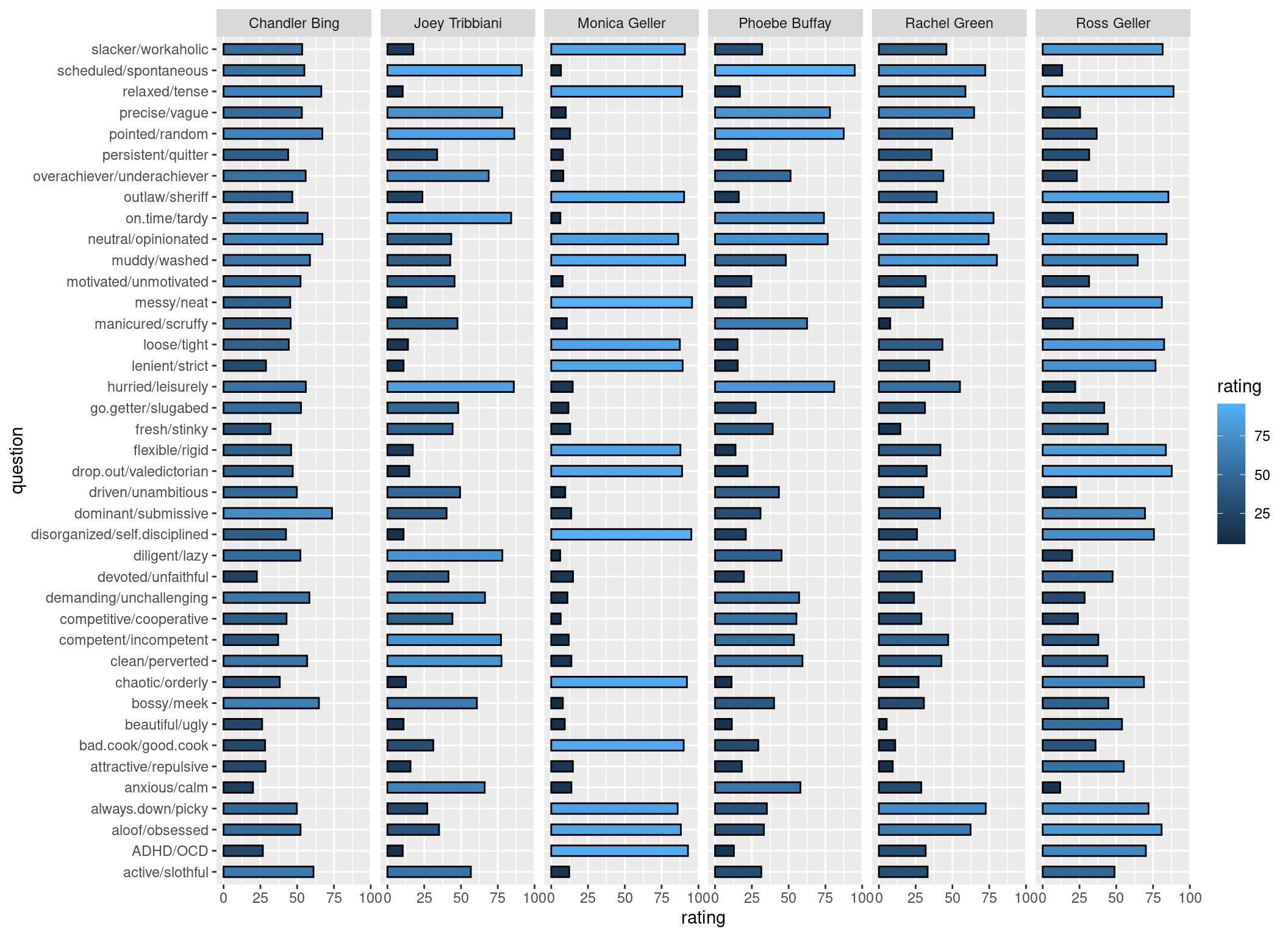

Style the plot. You could choose another color palette, another theme, other labels … Get creative!

Solution

p +
  scale_fill_viridis_c(option = "D") +
  theme_bw() +
  ggtitle("Characteristics of the 'Friends' characters") +
  xlab("Rating") +
  ylab("")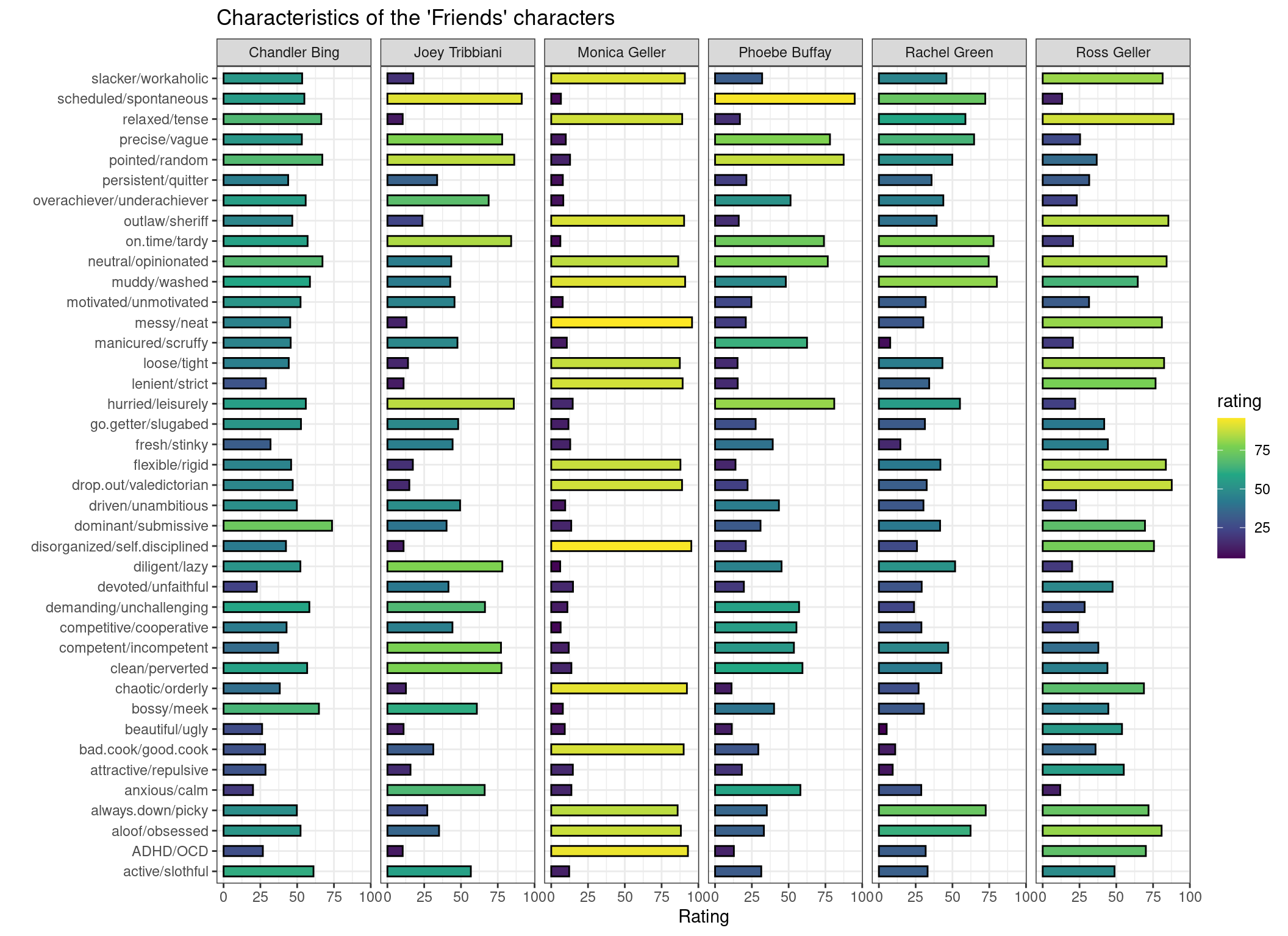

Great! With this color scale we can easily spot if a character is more balanced in his/her personality characteristics (like Chandler Bing), or tends to be pretty extreme (like Monica Geller or Joey Tribbiani).

Optional: Make a function out of it

Now, let’s make a function out of it, where you can input a fictional universe, the questions you are interested in, and receive a plot! Just merge together the code snippets you have created during this exercise, and test the function with some fictional universes of your choice.

Solution

fictional_personalities <- function(fictional_universe, questions) {
  ## Prepare the data:
  characters_plot <- characters_stats %>%
    mutate(question = gsub("_", "/", .$question)) %>%
    filter(
      uni_name == fictional_universe,
      question %in% questions
    )

  ## Merge together the code snippets we already saw in the other exercises.
  p <- ggplot(
    data = characters_plot,
    aes(
      x = rating,
      y = question
    )
  ) +
    facet_grid(. ~ name) +
    geom_col(
      aes(fill = rating),
      colour = "black",
      width = 0.5
    ) +
    scale_fill_viridis_c(option = "D") +
    theme_bw() +
    ggtitle(paste("Characteristics of the '", fictional_universe, "' characters")) + # paste together the title, so it always shows the correct fictional universe
    xlab("Rating") +
    ylab("")

  print(p)
}

Now, let’s try it out:

fictional_personalities(
  fictional_universe = "How I Met Your Mother",
  questions = unique(characters_stats$question)[1:20]
) # Use the first 40 questions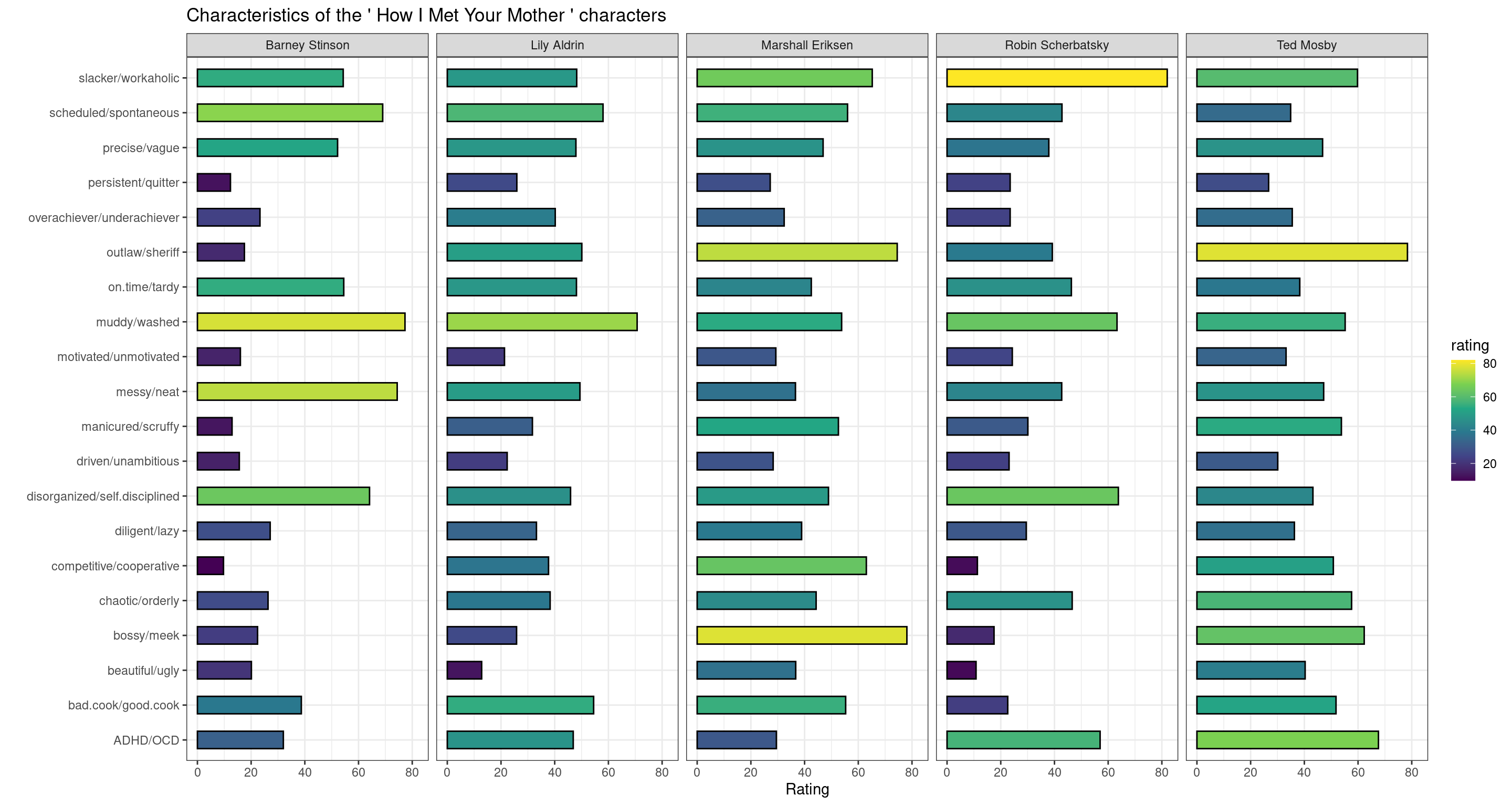

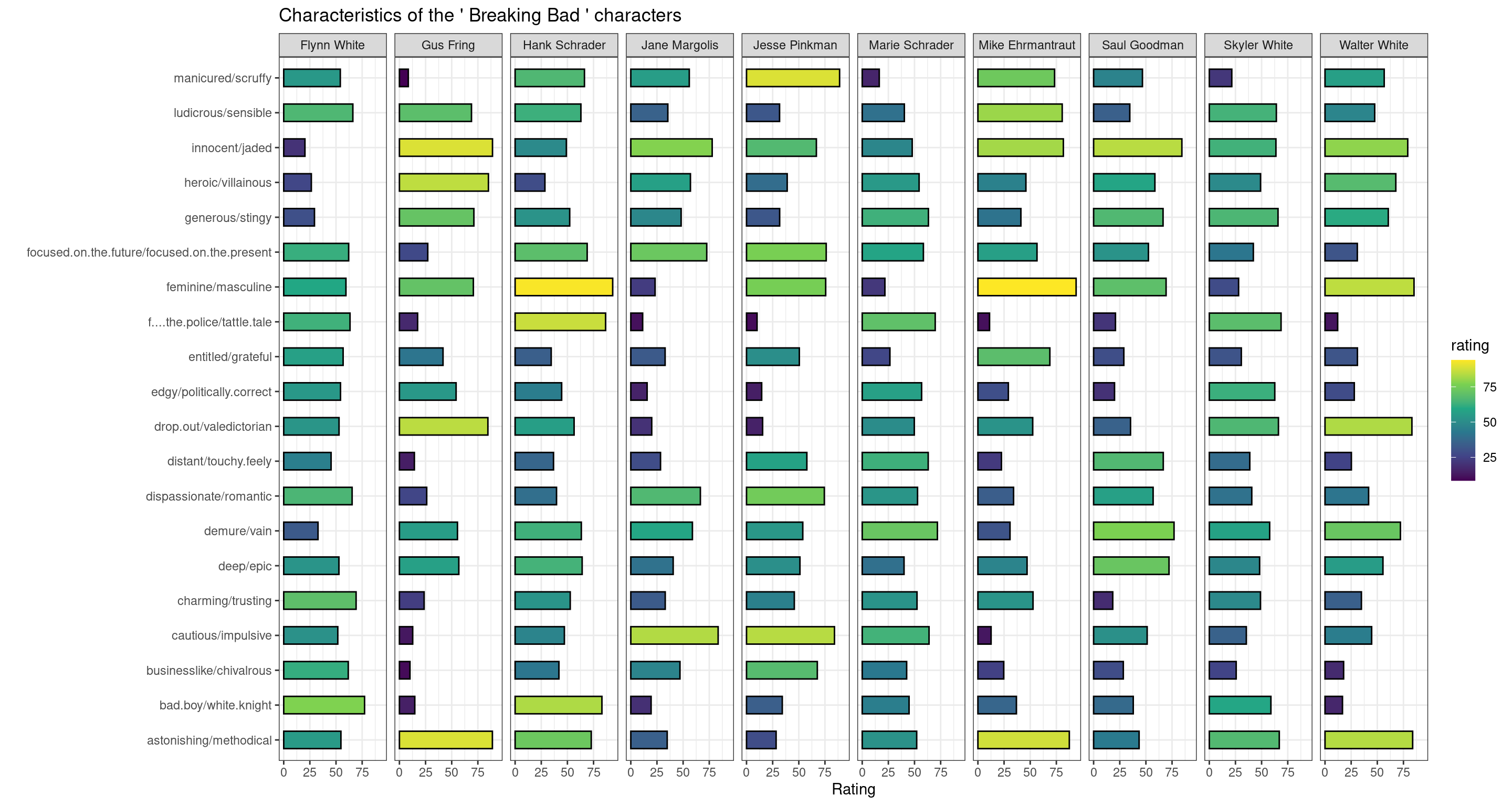
## Sample some questions randomly:
set.seed(42) # This makes the random sampling reproducable
random_questions <- sample(unique(characters_stats$question), 20)

fictional_personalities(
  fictional_universe = "Breaking Bad",
  questions = random_questions
)

The End

Amazing, you’ve made it to the end of this workshop! You now can go back to The Big Picture, or do the Final Exercise to test your knowledge one more time! If you had enough exercises for today, take a look at some of the Resources I have assembled for further reading.