Project Setup

We will start by setting up a simple example of a reproducible report.

Create Quarto Project

First, we will need to create a new Quarto project.

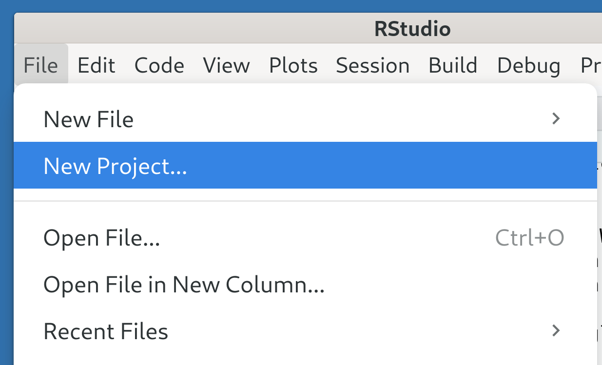
If you haven’t already, open RStudio – see Note 1 for how to use the terminal instead. Then, click on File > New Project… to open the New Project Wizard.

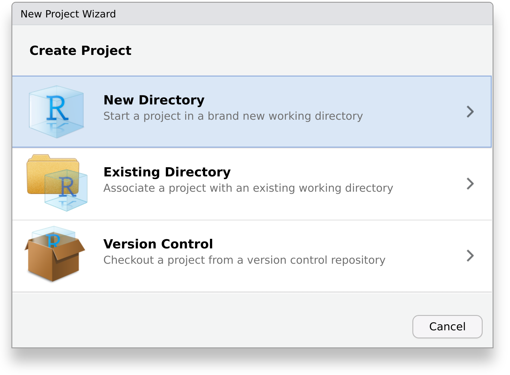
Here, select New Directory

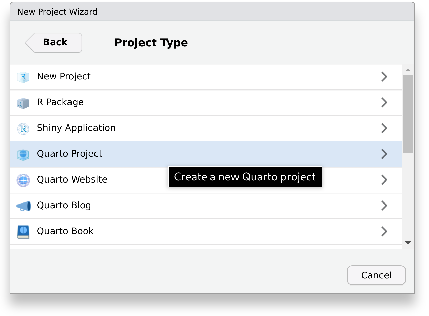
And choose the project type Quarto Project.

Finally, enter the name of the directory where our report will be created in, for example code-publishing-exercise.

As we will use Git to track the version history of files, be sure to check Create a git repository. If you don’t know what Git is, have a look at the tutorial “Introduction to version control with git and GitHub within RStudio”.

renv: A dependency management toolkit for R

Also, we will utilize the package renv to track the R packages our project depends on. Using it makes it easier for others to view and obtain them at a later point in time. Therefore make sure that the box Use renv with this project is checked. Again, if this is the first time you are hearing about renv, have a look at the tutorial “Introduction to {renv}”.

If you are already familiar with Markdown and Quarto, you can uncheck the box Use visual markdown editor.

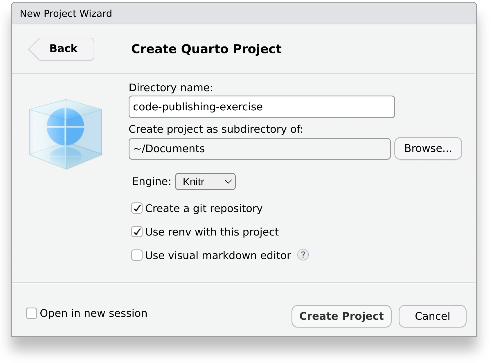
Click on Create Project. Your RStudio window should now look similar to this:

The project `code-publishing-exercise` opened in RStudio. The source pane to the top left has a Quarto file open called "code-publishing-exercise.qmd". The console pane to the bottom left indicates by its output that renv is active in the current project. The environment pane to the top right indicates that the environment is currently empty. The output pane to the bottom right shows the files in the current project.

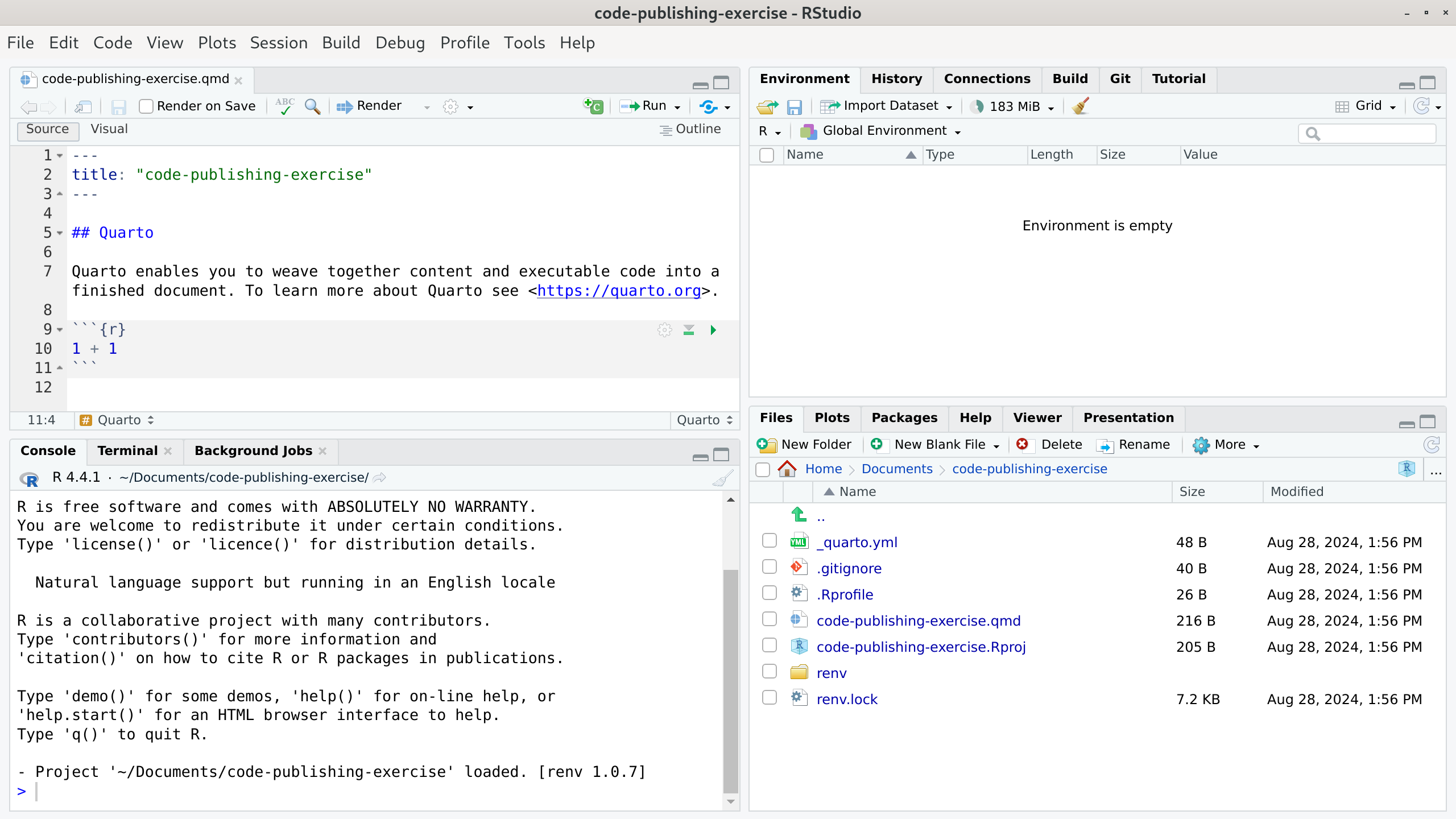
If, like in the image, a Quarto file with some demo content was opened automatically, you can close and delete it, for example, using RStudio’s file manager.

Make sure that your project is in a consistent state according to renv by running:

Console
renv::status()

If it reports packages that are not used, synchronize the lock file using:

Console
renv::snapshot()

Without RStudio, one can create a Quarto project with version control and renv enabled by typing the following into a terminal:

Terminal
quarto create project default code-publishing-exercise
cd code-publishing-exercise/
rm code-publishing-exercise.qmd
git init
git checkout -b main

Then, one can open an R session, by simply typing R into the terminal. Next, make sure that getwd() indicates that the working directory is code-publishing-exercise. If not, set it using setwd("code-publishing-exercise"). Then, initialize renv:

Console
renv::init()

You are now ready to stage and commit your files. You can either stage files separately or the whole project folder at once. If you do the latter, we recommend you to inspect the untracked changes before staging all of them:

In file paths, a period (.) means “the current directory”, while two periods (..) mean “the parent directory”. Therefore git add . means “stage the current directory for committing”.

Terminal
git status

Since no commits have been made so far, this should include every file that is not covered by the .gitignore file. If everything can be staged for committing – as is the case in this tutorial – you can follow up with:

Terminal
git add .
git commit -m "Initial commit"

If you see a file you’d rather not commit, delete it or add its name to the .gitignore file. If you don’t check your changes before committing, you might accidentally commit something you’d rather not.

Tip 1

If git commit fails with the message Author identity unknown, you need to tell Git who you are. Run the following commands to set your name and email address:

Terminal
git config user.name "YOUR NAME"
git config user.email "YOUR EMAIL ADDRESS"

Then, commit again.

Decide on Structure

Before adding your project files, it is helpful to decide on a directory structure, that is, how to call each file and where to put it. In general, the directory structure should facilitate understanding a project by breaking it into logical chunks. There is no single best solution, as a good structure depends on where a project’s complexity lies. However, it is usually helpful if the different files and folders reflect the execution order. For example, if there are multiple data processing stages, one can possibly differentiate input (raw data), intermediate (processed data), and output files (e.g., figures) and put them into separate folders. Similarly, the corresponding code files (e.g., preparation, modeling, visualization) can be prefixed with increasing numbers.

Luckily, there are already numerous proposals for how to organize one’s project files, both general (e.g., Wilson et al. 2017; Project TIER 2021) as well as specific to a particular programming language (e.g., Marwick, Boettiger, and Mullen 2018; Vuorre and Crump 2021) or journal (Vilhuber 2021). We recommend you to follow the standards of your field.
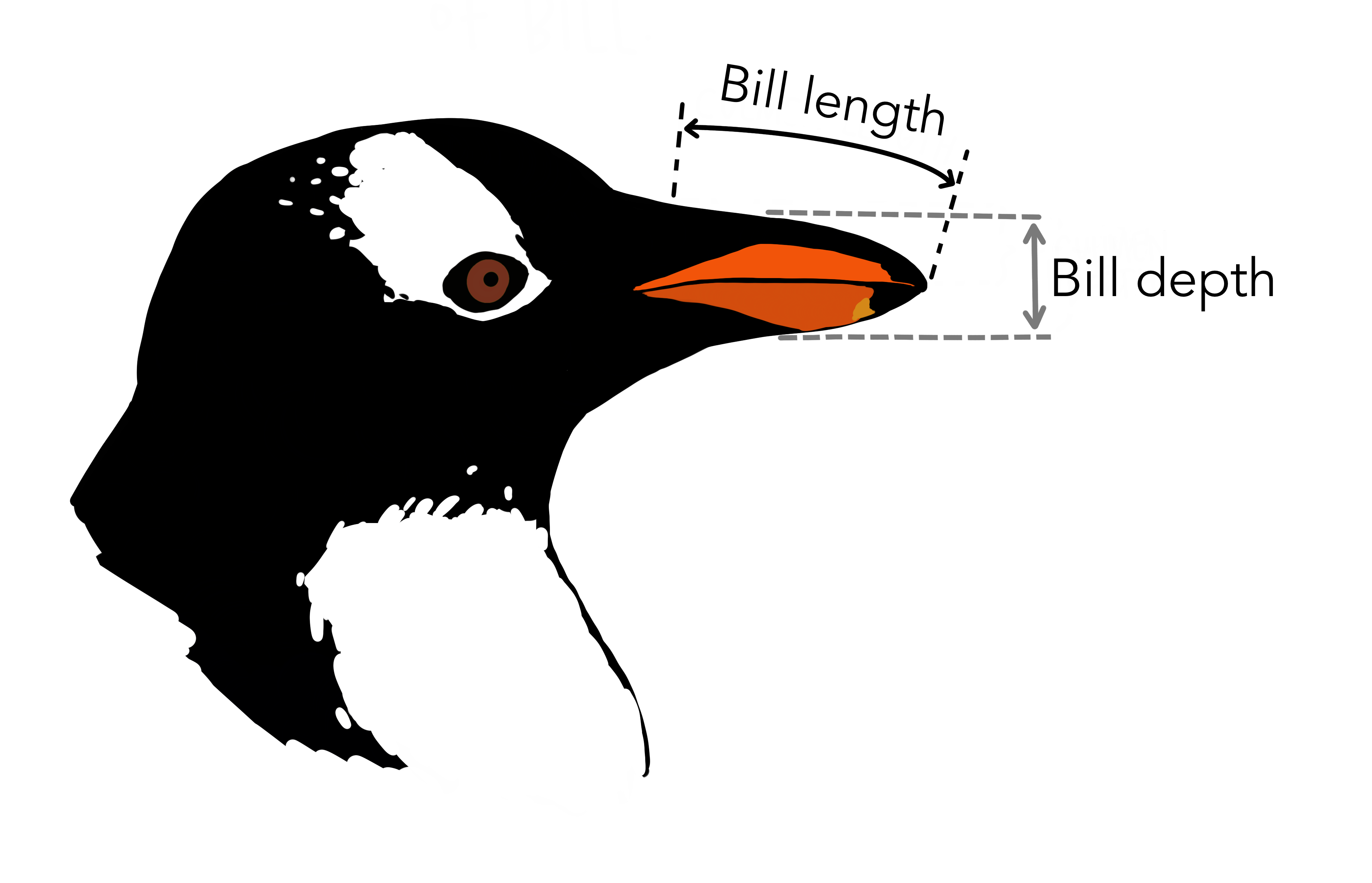
For the purpose of this tutorial, we will provide you with a data set and a corresponding analysis. They are simple enough to be put together in the root folder of your project.

Add Data

You can now download the data set we have prepared for you and put into your project folder: Data.csv

palmerpenguins: Palmer Archipelago (Antarctica) Penguin Data

The data set is from the package palmerpenguins and contains the recorded bill lengths and sex of penguins living on three islands in the Palmer Archipelago, Antarctica. It was made available under the license CC0 1.0.

When publishing a data set, it is important to document the meaning (e.g., units) and possible values of its variables. This is typically done with a data dictionary (also called a codebook). In the following, we will demonstrate how to create a simple data dictionary using the R packages tinylabels, datawizard, and tinytable. You can install them now using:

Console
renv::install(c(
  "tinylabels",
  "datawizard",
  "tinytable"
))

You can put the code that follows for creating the data dictionary into a new file called create_data_dictionary.R.

Using tinylabels we can add labels to the variables of a data.frame in R:2

create_data_dictionary.R
## dat <- read.csv("Data.csv")

descriptions <- c(
  species = "a character string denoting penguin species",
  island = "a character string denoting island in Palmer Archipelago, Antarctica",
  bill_length_mm = "a number denoting bill length (millimeters)",
  bill_depth_mm = "a number denoting bill depth (millimeters)",
  flipper_length_mm = "an integer denoting flipper length (millimeters)",
  body_mass_g = "an integer denoting body mass (grams)",
  sex = "a character string denoting penguin sex",
  year = "an integer denoting the study year"
)
tinylabels::variable_label(dat) <- descriptions

Subsequently, datawizard can be employed to create the data dictionary containing the name and label, but also some other information about each variable:

datawizard: Easy Data Wrangling and Statistical Transformations
create_data_dictionary.R
(dict <- datawizard::data_codebook(dat) |>
  subset(select = -.row_id) |>
  tinytable::tt())
ID Name Label Type Missings Values N Prop
1 species a character string denoting penguin species character 0 (0.0%) Adelie 152 44.2%
Chinstrap 68 19.8%
Gentoo 124 36.0%
2 island a character string denoting island in Palmer Archipelago, Antarctica character 0 (0.0%) Biscoe 168 48.8%
Dream 124 36.0%
Torgersen 52 15.1%
3 bill_length_mm a number denoting bill length (millimeters) numeric 2 (0.6%) [32.1, 59.6] 342
4 bill_depth_mm a number denoting bill depth (millimeters) numeric 2 (0.6%) [13.1, 21.5] 342
5 flipper_length_mm an integer denoting flipper length (millimeters) integer 2 (0.6%) [172, 231] 342
6 body_mass_g an integer denoting body mass (grams) integer 2 (0.6%) [2700, 6300] 342
7 sex a character string denoting penguin sex character 11 (3.2%) female 165 49.5%
male 168 50.5%
8 year an integer denoting the study year integer 0 (0.0%) 2007 110 32.0%
2008 114 33.1%
2009 120 34.9%

Finally, we can store the data dictionary inside an HTML file using the R package tinytable and put the HTML file into the project folder as well.

tinytable: Simple and Configurable Tables
create_data_dictionary.R
tinytable::save_tt(dict, output = "data_dictionary.html")

A human-readable data dictionary is necessary for making one’s research reproducible and the example we provided demonstrates only the bare minimum. A full data documentation including measurement instruments, sampling procedures, appropriate weighting, contact information, and more information about the study can be created with the R package pointblank. And one could go even further by making the information machine-readable in a standardized way. We provide an optional example of that in Note 2. If you want to learn more about the sharing of research data, have a look at the tutorial “FAIR research data management”.

This example demonstrates how the title and description of the data set, the description of the variables and their possible values are stored in a machine-readable way.

table_info <- c(
  title = "penguins dataset",
  description = "Size measurements for adult foraging penguins near Palmer Station, Antarctica"
)
descriptions <- c(
  species = "a character string denoting penguin species",
  island = "a character string denoting island in Palmer Archipelago, Antarctica",
  bill_length_mm = "a number denoting bill length (millimeters)",
  bill_depth_mm = "a number denoting bill depth (millimeters)",
  flipper_length_mm = "an integer denoting flipper length (millimeters)",
  body_mass_g = "an integer denoting body mass (grams)",
  sex = "a character string denoting penguin sex",
  year = "an integer denoting the study year"
)
vals <- list(
  species = c("Adelie", "Gentoo", "Chinstrap"),
  island = c("Torgersen", "Biscoe", "Dream"),
  sex = c("male", "female"),
  year = c(2007, 2008, 2009)
)

Generally, metadata are either stored embedded into the data or externally, for example, in a separate file. We will use the “frictionless data” standard, where metadata are stored separately.

Specifically, one can use the R package frictionless to create a schema which describes the structure of the data. For the purpose of the following code, it is just a nested list that we edit to include our own information. We also explicitly record in the schema that missing values are stored in the data file as NA and that the data are licensed under CC0 1.0. Finally, the package is used to create a metadata file that contains the schema.

# Read data and create schema
dat_filename <- "Data.csv"
dat <- read.csv(dat_filename)
dat_schema <- frictionless::create_schema(dat)

# Add descriptions to the fields
dat_schema$fields <- lapply(dat_schema$fields, \(x) {
  c(x, description = descriptions[[x$name]])
})

# Record possible values
dat_schema$fields <- lapply(dat_schema$fields, \(x) {
  if (x$name %in% names(vals)) {
    modifyList(x, list(constraints = list(enum = vals[[x$name]])))
  } else {
    x
  }
})

# Define missing values
dat_schema$missingValues <- c("", "NA")

# Create package with license info and write it
dat_package <- frictionless::create_package() |>
  frictionless::add_resource(
    resource_name = "penguins",
    data = dat_filename,
    schema = dat_schema,
    title = table_info[["title"]],
    description = table_info[["description"]],
    licenses = list(list(
      name = "CC0-1.0",
      path = "https://creativecommons.org/publicdomain/zero/1.0/",
      title = "CC0 1.0 Universal"
    ))
  )
frictionless::write_package(dat_package, directory = ".")

This creates the metadata file datapackage.json in the current directory. Make sure it is located in the same folder as Data.csv, as together they comprise a data package.

Having added the data and its documentation, one can view and record the utilized packages with renv

Console
renv::status()
renv::snapshot()

…and go through the commit routine:

Terminal
git status
git add .
git commit -m "Add data"

Add Code

In order to have some code which you can practice to share, we have prepared a simple manuscript for you, alongside a bibliography file. The manuscript contains code together with a written narrative. Download the two files to your computer and put them into your project folder.

The manuscript explores differences in bill length between male and female penguins, feel free to read through it.

As the manuscript uses some new packages, install them with:

Console
renv::install()

The manuscript also uses the Quarto extension “apaquarto”, which typesets documents according to the requirements of the American Psychological Association (2020). It can be installed in the project using the following command:

Terminal
quarto add --no-prompt wjschne/apaquarto
Tip 2: Not a psychologist?

If you are not a psychologist, you can also skip installing apaquarto. If you installed it by accident, run quarto remove wjschne/apaquarto.

Note, however, that the file Manuscript.qmd we prepared for you uses apaquarto by default and you need to set a different format in the YAML header if you decide not to use apaquarto:

Manuscript.qmd
format:
  pdf:
    pdf-engine: lualatex
    documentclass: scrartcl
    papersize: a4

Also, you need to have a \(\TeX\) distribution installed on your computer, which is used in the background to typeset PDF documents. A lightweight choice is TinyTeX, which can be installed with Quarto as follows:

Terminal
quarto install tinytex

You should now be able to render the document using Quarto:

Terminal
quarto render Manuscript.qmd

This should create a PDF file called Manuscript.pdf in your project folder.

Tip 3

If the PDF file cannot be created, try updating Quarto. It comes bundled with RStudio, however apaquarto sometimes requires more recent versions.

With the code being added, one can use renv again to view and record the new packages:

Console
renv::status()
renv::snapshot()
Tip 4

Always run renv::status() and resolve any inconsistencies before you commit code to your project. This way, every commit represents a working state of your project.

Finally, make your changes known to Git:

Terminal
git status
git add .
git commit -m "Add manuscript"
Warning 3: Beware of Credentials

Sometimes, a data analysis requires the interaction with online services:

  • Data may be collected from social network sites using their APIs3 or downloaded from a data repository, or
  • an analysis may be conducted with the help of AI providers.

In these cases, make sure that the code you check in to Git does not contain any credentials that are required for accessing these services. Instead, make use of environment variables which are defined in a location that is excluded from version control. When programming with R, you can define them in a file called .Renviron in the root of your project folder:

.Renviron
MY_FIRST_KEY="your_api_key_here"
MY_SECOND_KEY="your_api_key_here"

When you start a new session from the project root, the file is automatically read by R and the environment variables can be accessed using Sys.getenv():

query_api(..., api_key = Sys.getenv("MY_FIRST_KEY"))

Make sure that .Renviron is added to your .gitignore file in order to exclude it from the Git repository. If you already committed a file that contains credentials, you can follow Chacon and Straub (2024).

Coding Best Practices

Although we provide the code in this example for you, a few things remain to be said about best practices when it comes to writing code that is readable and maintainable.

  • Use project-relative paths. When you refer to a file within your project, write paths relative to your project root. For example, don’t write C:/Users/Public/Documents/my_project/images/result.png, instead write images/result.png.

  • Keep it simple. Add complexity only when you must. Whenever there’s a boring way to do something and a clever way, go for the boring way. If the code grows increasingly complex, refactor it into separate functions and files.

  • Don’t repeat yourself. Use variables and functions before you start to write (or copy-paste) the same thing twice.

  • Use comments to explain why you do things. The code already shows what you do. Use comments to summarize it and explain why you do it.

  • Don’t reinvent the wheel. With R, chances are that what you need to do is greatly facilitated by a package from one of many high-quality collections such as rOpenSci, r-lib, Tidyverse, or fastverse.

  • Think twice about your dependencies. Every dependency increases the risk of irreproducibility in the future. Prefer packages that are well-maintained and light on dependencies4. We also recommend you to read “When should you take a dependency?” by Wickham and Bryan (2023).

  • Fail early, often and noisily. Whenever you expect a certain state, use assertions to be sure. In R, you can use stopifnot() to make sure that a condition is actually true.

  • Test your code. Test your code with scenarios where you know what the result should be. Turn bugs you discovered into test cases. Use linting tools5 to identify common mistakes in your code, for example, the R package lintr.

  • Read through a style guide and follow it. A style guide is a set of stylistic conventions that improve the code quality. R users are recommended to read Wickham’s (2022) “Tidyverse style guide” and use the R package styler. Python users may benefit from reading the “Style Guide for Python Code” by Rossum, Warsaw, and Coghlan (2013). And even if you don’t follow a style guide, be consistent.

This is only a brief summary and there is much more to be learned about coding practices. If you want to dive deeper we recommend the following resources:

“Any fool can write code that a computer can understand. Good programmers write code that humans can understand.”

— Martin Fowler, British software engineer

The Last Mile

renv only records the versions of R packages and of R itself. This means that potential system dependencies of R packages and other tools utilized in the project are not documented anywhere, including Quarto.6 We will manually write them down when creating a README. For now, however, there is one simple step you can take to record the version of Quarto (and a few other dependencies). Do run the following:

Terminal
quarto use binder

This will create a few additional files which facilitate reconstructing the computational environment in the future.7 As always, commit your changes:

Terminal
git status
git add .
git commit -m "Add repo2docker config"

You are now all set up to prepare your project for sharing!

Back to top

References

Chacon, Scott, and Ben Straub. 2024. “Removing a File from Every Commit.” In Pro Git, Second edition. Apress. https://git-scm.com/book/en/v2/Git-Tools-Rewriting-History#_removing_file_every_commit.
Marwick, Ben, Carl Boettiger, and Lincoln Mullen. 2018. “Packaging Data Analytical Work Reproducibly Using R (and Friends).” The American Statistician 72 (1): 80–88. https://doi.org/10.1080/00031305.2017.1375986.
Mineault, Patrick, and Kento Nozawa. 2021. “The Good Research Code Handbook.” https://goodresearch.dev/. December 21, 2021. https://doi.org/10.5281/ZENODO.5796873.
Project TIER. 2021. TIER Protocol 4.0.” 2021. https://www.projecttier.org/tier-protocol/protocol-4-0/.
Publication Manual of the American Psychological Association. 2020. 7th ed. Washington: American Psychological Association. https://doi.org/10.1037/0000165-000.
Raymond, Eric S. 2003. The Art of UNIX Programming: With Contributions from Thirteen UNIX Pioneers, Including Its Inventor, Ken Thompson. Addison-Wesley Professional Computing Series. Boston: Addison-Wesley. https://www.arp242.net/the-art-of-unix-programming/.
Rossum, Guido van, Barry Warsaw, and Alyssa Coghlan. 2013. “Style Guide for Python Code. Python Enhancement Proposals (PEPs).” August 1, 2013. https://peps.python.org/pep-0008/.
Vilhuber, Lars. 2021. “Preparing Your Files for Verification. Office of the AEA Data Editor.” April 8, 2021. https://aeadataeditor.github.io/aea-de-guidance/preparing-for-data-deposit.
Vuorre, Matti, and Matthew J. C. Crump. 2021. “Sharing and Organizing Research Products as R Packages.” Behavior Research Methods 53 (2): 792–802. https://doi.org/10.3758/s13428-020-01436-x.
Wickham, Hadley. 2022. “The Tidyverse Style Guide.” July 24, 2022. https://style.tidyverse.org/.
———. 2023. “Tidy Design Principles.” November 20, 2023. https://design.tidyverse.org/.
Wickham, Hadley, and Jennifer Bryan. 2023. “When Should You Take a Dependency?” In R Packages, Second edition. O’Reilly Media. https://r-pkgs.org/dependencies-mindset-background.html#sec-dependencies-pros-cons.
Wilson, Greg, Jennifer Bryan, Karen Cranston, Justin Kitzes, Lex Nederbragt, and Tracy K. Teal. 2017. “Good Enough Practices in Scientific Computing.” PLOS Computational Biology 13 (6): 1–20. https://doi.org/10.1371/journal.pcbi.1005510.

Footnotes

  1. For example, using Amnesia, ARX, sdcMicro, or Synthpop.↩︎

  2. Note that the code provided does not alter the data file – no labels will be added to Data.csv. The labels are only added to a (temporary) copy of the data set within R in order to create the data dictionary.↩︎

  3. An application programming interface provides the capability to interact with other software using a programming language.↩︎

  4. You can use the function pak::pkg_deps() to count the total number of package dependencies in R.↩︎

  5. A linting tool analyzes your code without actually running it. This process is called static code analysis.↩︎

  6. As of August 2024, a proposal to record the version of Quarto has not been implemented, see rstudio/renv#1143.↩︎

  7. Either using repo2docker or the public binder service.↩︎