Real-life example
This is a walk through one relatively simple simulation written to check whether the following two models would provide the same results:
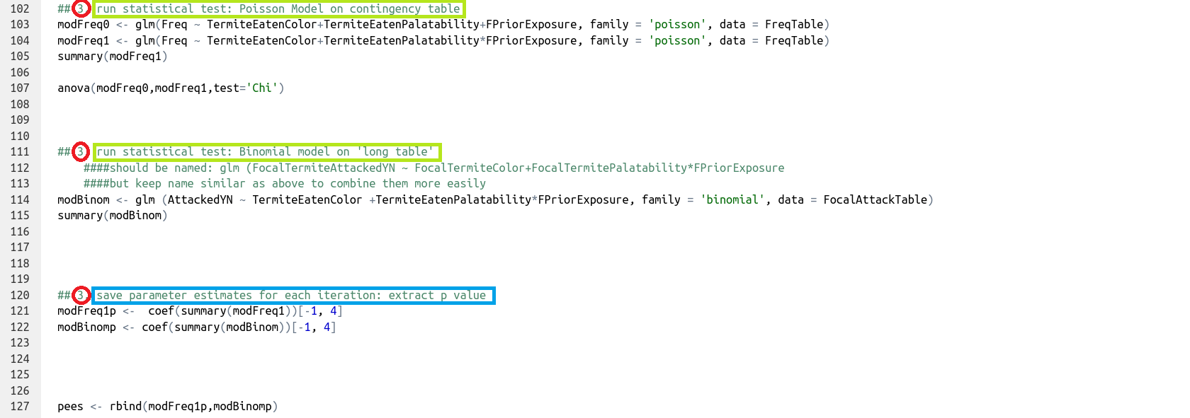
- A generalized linear model based on a contingency table of counts (Poisson distribution).
- A generalized linear model with one line per observation and the occurrence of the variable of interest coded as ‘Yes’ or ‘No’ (binomial distribution).
I created this code while preparing my preregistration for a simple behavioural ecology experiment about methods for independently manipulating palatability and colour in small insect prey (article, OSF preregistration).
The R script screenshot below, glm_Freq_vs_YN.R, can be found in the folder Ihle2020.
This walkthrough will use the steps as defined on the page ‘General structure’.
Define sample sizes (within a dataset and number of repetitions), experimental design (fixed dataset structure, e.g. treatment groups, factors), and parameters that will need to vary (here, the strength of the effect).
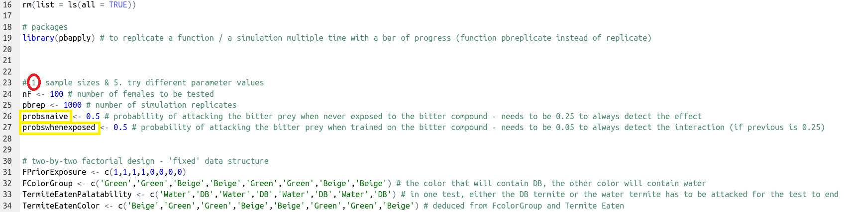
Generate data (here, using
sample()and the probabilities defined in step 1) and format it in two different ways to accommodate the two statistical tests to be compared.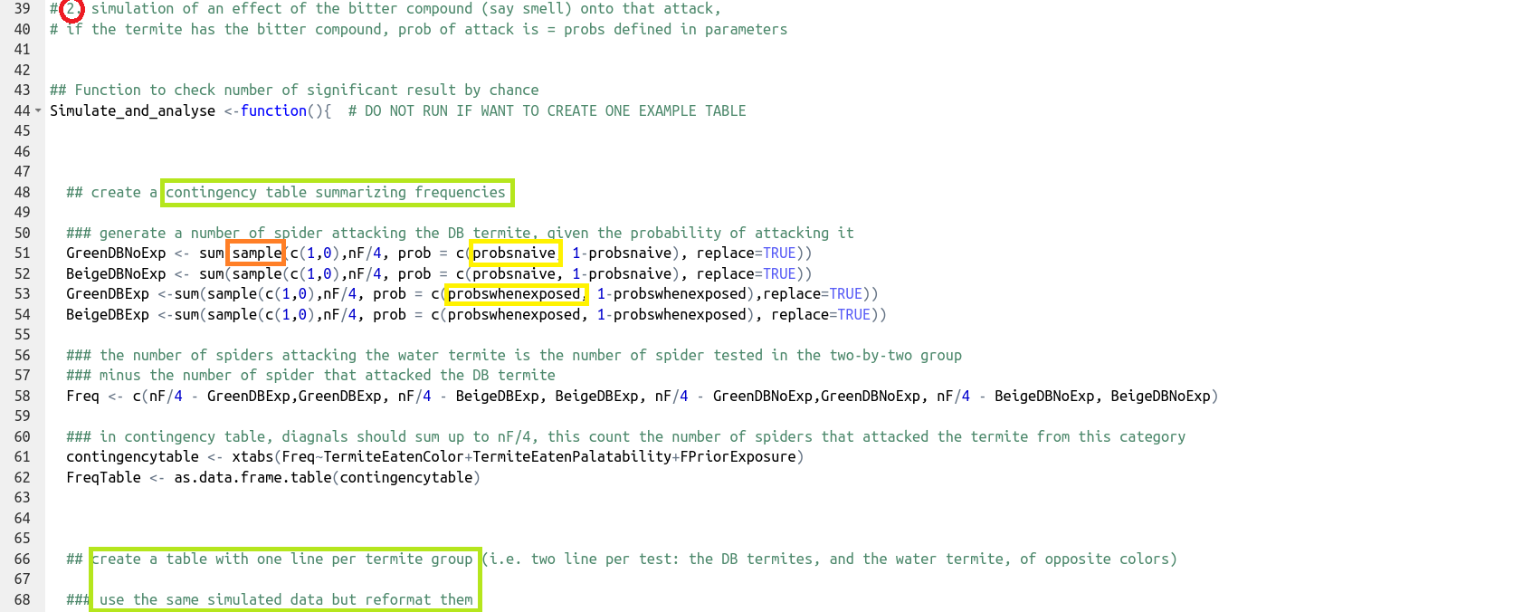
Run the statistical test and save the parameter estimate of interest for that iteration. Here, this is done for both statistical tests to be compared.
Repeat steps 2 (data simulation) and 3 (data analyses) to get the distribution of the parameter estimates by wrapping these steps in a function.
Definition of the function at the beginning:

Output returned from the function at the end:

Repeat the functionnreptimes. Here,pbreplicate()is used to provide a bar of progress for R to run this command.

Explore the parameter space. Here, vary the probabilities of sampling between 0 and 1 depending on the treatment group category.

Analyse and interpret the combined results of many simulation repetitions. In this case, the results of the two models were qualitatively the same (comparison of results for a few different parameter values), and both models gave the same expected 5% false positive results when no effect was simulated. Varying the effect (the probability of sampling 0 or 1 depending on the experimental treatment) allowed us to find the minimum effect size for which the number of positive results of the tests is over 80%.