Checking power through simulations

The power of a statistical test tells us the probability that the test correctly rejects the null hypothesis. In other words, if we only examine true effects, the power is the proportion of tests that will (correctly) reject the null hypothesis. Often, the power is set to 80%, though, as with \(\alpha = .05\), this is an arbitrary choice.

Generally, we want to do a power analysis before collecting data, to work out the sample size we need to detect some effect with a sufficient probability. If we are calculating a required sample size, the analysis is called “a priori power analyses”, or simply “sample size calculation”.

Taking the example of a t-test, we need to understand a few parameters:

• n, the sample size.
• delta, the difference in means that you want to be able to detect. Deciding what this value should be is tricky. You might rely on estimates from the literature (though bear in mind they are likely to be inflated), or you can use a minimally important difference, which is the threshold below which you do not consider a difference interesting enough to be worth detecting. In a clinical trial, for example, this might be the smallest difference that a patient would care about.
• sd, the standard deviation. Usually, this needs to be estimated from the literature or pilot studies.
• sig.level, the \(\alpha\), as discussed previously.
• power, the power as defined above.

You can calculate any one of these parameters, given all of the others. In an a-priori power analysis, we need to specify delta, sd, sig.level and power to calculate the required sample size:

power.t.test(n = NULL, delta = 0.5, sd = 1, sig.level = 0.05, power = 0.8)

Notice that n = NULL, so this parameter is calculated and returned by the function.

The sample size n we need, given this set of parameters, is 64 per group.

Just as we can check the \(\alpha\) of our test by sampling from the same distribution (i.e., simulating data without an effect), we can check the power by sampling from different distributions (i.e., simulating data with an effect).

If we sample values from two normal distributions with different means (e.g. \(N(0,1)\) and \(N(0.5,1)\)), what is the minimum sample size we need to detect a significant difference in means with a t-test 80% of the time?

---

YOUR TURN:

1. Use your simulation skills to work out the power through simulation. Write a function that does the following:

   1. Draw n values from a random normal distribution with mean1 and another n values from a normal distribution with mean2.
   2. Compare the means of these two samples with a t-test and extract the p-value.

2. Repeat the function 1000 times using the parameters used in the power calculation above (that used the power.t.test() function).

3. Calculate the proportion of p-values that are smaller than 0.05.

---

p-values of t-tests comparing means from 1000 repetitions simulating \(N(0,1)\) and \(N(0.5,1)\) with n = 64:

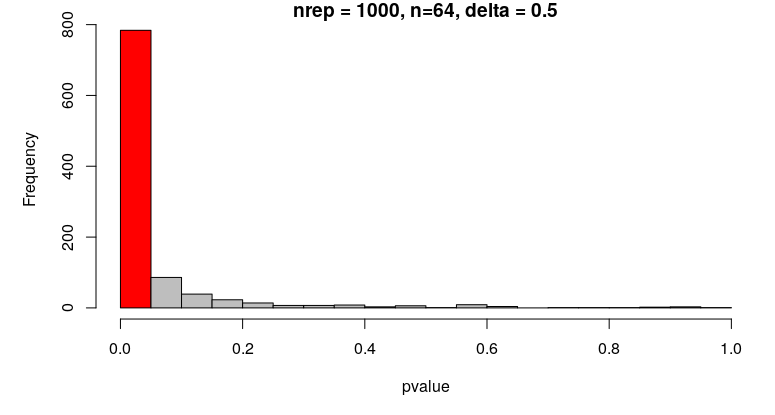
The proportion of correctly rejected null hypotheses in the simulation is close to 0.8, which is what we would expect:

Using simulations for power analysis is not really necessary for simple examples like a t-test, though it is useful to check your understanding.

When analyses become complex and it is hard or impossible to determine a sample size analytically (i.e. you can’t calculate it, or there’s no suitable function to use), then simulations are an indispensable tool.

A simple example of a power analysis like the one you’ve just done can be found in the “Power analysis” section of this paper:

• Blanco, D., Schroter, S., Aldcroft, A., Moher, D., Boutron, I., Kirkham, J. J., & Cobo, E. (2020). Effect of an editorial intervention to improve the completeness of reporting of randomised trials: a randomised controlled trial. BMJ Open, 10(5), e036799. https://doi.org/10.1136/bmjopen-2020-036799

A complete self-paced tutorial to simulate data for power analysis of complex statistical designs can be found here:

• https://lmu-osc.github.io/Simulations-for-Advanced-Power-Analyses/

---