library(knitr)
library(vsp)
library(Matrix)
library(scales)
Important
This document is an updated copy of a published commentary, to showcase Quarto manuscripts in our Quarto workshop. The official online repository of our published commentary can be found here.
A Short Commentary on Rohe & Zeng (2023)
In their paper “Vintage factor analysis with varimax performs statistical inference”, Rohe and Zeng [R&Z; Rohe & Zeng (2023)] demonstrate the usefulness of principal component analysis with varimax rotation (PCA+VR), a combination they call vintage factor analysis. The authors show that PCA+VR can be used to estimate factor scores and factor loadings, if a certain leptokurtic condition is fulfilled that can be assessed by simple visual diagnostics. In a side result, they also imply that PCA+VR is able to estimate factor scores even if the latent factors are correlated. In our commentary “New Insights into PCA + Varimax for Psychological Researchers” (Pargent et al., 2023), we briefly discuss some implications of these results for psychological research and note that the suggested diagnostics of “radial streaks” might give less clear results in typical psychological applications. The commentary includes extensive electronic supplemental materials, containing a data example and a small simulation on estimating correlated factors, that can be found at https://osf.io/5symf/.
In the current electronic supplementary materials, we present i) an exemplary data analysis that is discussed in our comment, and ii) a small simulation demonstrating the ability of PCA+VR to estimate correlated factors.
Data Example: The PhoneStudy
In [1]:
In contrast to the examples in R&Z which only deal with sparse binary network data, psychological applications (traditionally) deal with i) questionnaire items or (increasingly) ii) digital data, e.g., mobile sensing. The \(A\) matrix consists of i) integer-valued responses on \(d\) Likert items or ii) continuous values on \(d\) sensing variables, by \(n\) persons. Degree normalization discussed by R&Z does not seem suitable here and z-standardization is often required to detect meaningful factors in practice. We also do not share R&Z’s enthusiasm that “radial streaks” are common.
For the following demonstration, we use the publicly available PhoneStudy behavioral patterns dataset, which has been used to predict human personality from smartphone usage data (Stachl et al., 2020). The PhoneStudy collected i) self-reported questionnaire data of personality traits measured with the German Big Five Structure Inventory [BFSI; 5 factors and 30 facets, Arendasy et al. (2011)], ii) demographic variables (age, gender, education), and iii) behavioral data from smartphone sensing (e.g., communication & social behavior, app-usage, music consumption, overall phone usage, day-nighttime activity), bundled from several smaller studies. The mobile sensing data was recorded for up to 30 days on the personal smartphone of study volunteers.
Item responses to the personality questionnaire are contained in the file datasets/Items.csv while aggregated smartphone sensing variables are contained in the file datasets/clusterdata.RDS. Both can be downloaded from https://osf.io/fxv3k/download. We include copies of the aggregated datasets in our project repository for convenience. More details on the PhoneStudy data can be found in Stachl et al. (2020). Mobile sensing variables are described in more detail at https://compstat-lmu.shinyapps.io/Personality_Prediction/#section-datadict.
Item Response Data
Item responses to the 300 personality items of the Big Five questionnaire are almost complete and we decided to use complete case analysis here, although imputation would be possible as well.
In [2]:
phonedata_items = read.csv2("datasets/Items.csv")
phonedata_items = na.omit(phonedata_items[, 3:302])
As is common for psychometric analyses, we standardize the item response data with scale and convert the data.frame to a dgCMatrix that can be analyzed with vsp R package. However, not standardizing the items does not change the following results much here because there cannot be large outliers in item responses and item variances due to the fixed response format (all items are measured on a Likert scale with 4 labeled categories).
In [3]:
items_mat_z = as.matrix(scale(phonedata_items))
colnames(items_mat_z) = colnames(phonedata_items)
items_mat_z = as(items_mat_z, "dgCMatrix")
The screeplot suggests a decrease in singular values after the 5th component. This is in line with the theory behind the questionnaire that was constructed to measure the Big Five personality factors.
In [4]:
screeplot(vsp(items_mat_z, rank = 50,
  degree_normalize = FALSE, center = FALSE))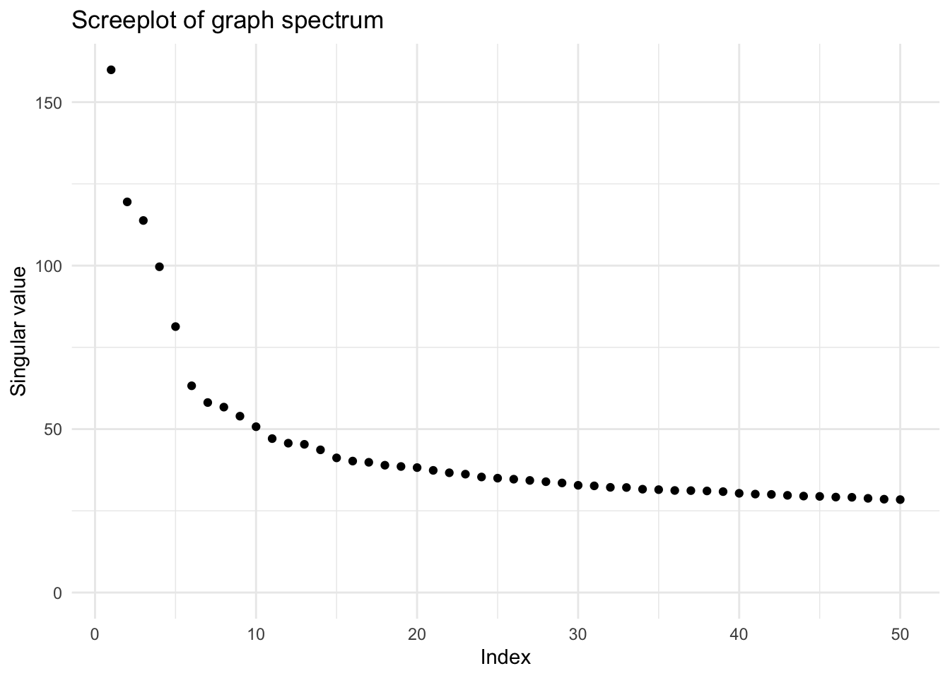
Note that each Big Five factor is represented in the questionnaire by 6 lower order personality facets measured by 10 items each. Thus, theory would suggest that extracting 30 components should also be meaningful.
To keep it simple, we extract only 5 components here.
In [5]:
pca_items_z = vsp(items_mat_z, rank = 5,
  degree_normalize = FALSE, center = FALSE)
Note that we do set degree_normalize = FALSE and center = FALSE because we do not analyze binary network data and we have already standardized our item responses.
We search for radial streaks in the estimated component and loading matrices:
In [6]:
pairs(as.matrix(pca_items_z$Z[, 1:5]), cex = 0.5, col = alpha("red", alpha = 0.2),
  main = "Estimated components (with standardization)")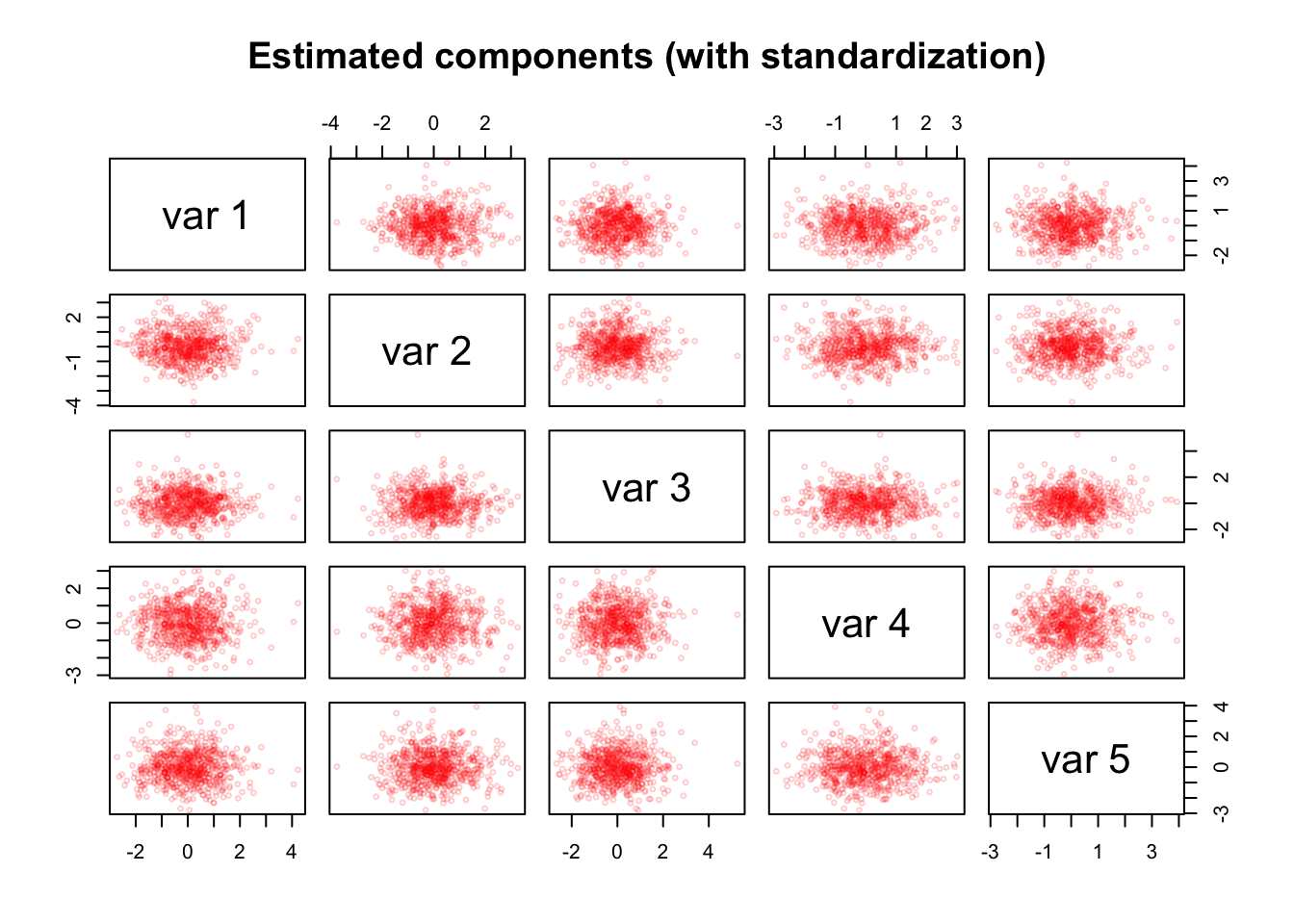
We do not find streaks in the estimated component matrix \(\hat{Z}\).
In [7]:
pairs(as.matrix(pca_items_z$Y[, 1:5]), cex = 0.5, col = alpha("red", alpha = 0.3),
  main = "Estimated loadings (with standardization)")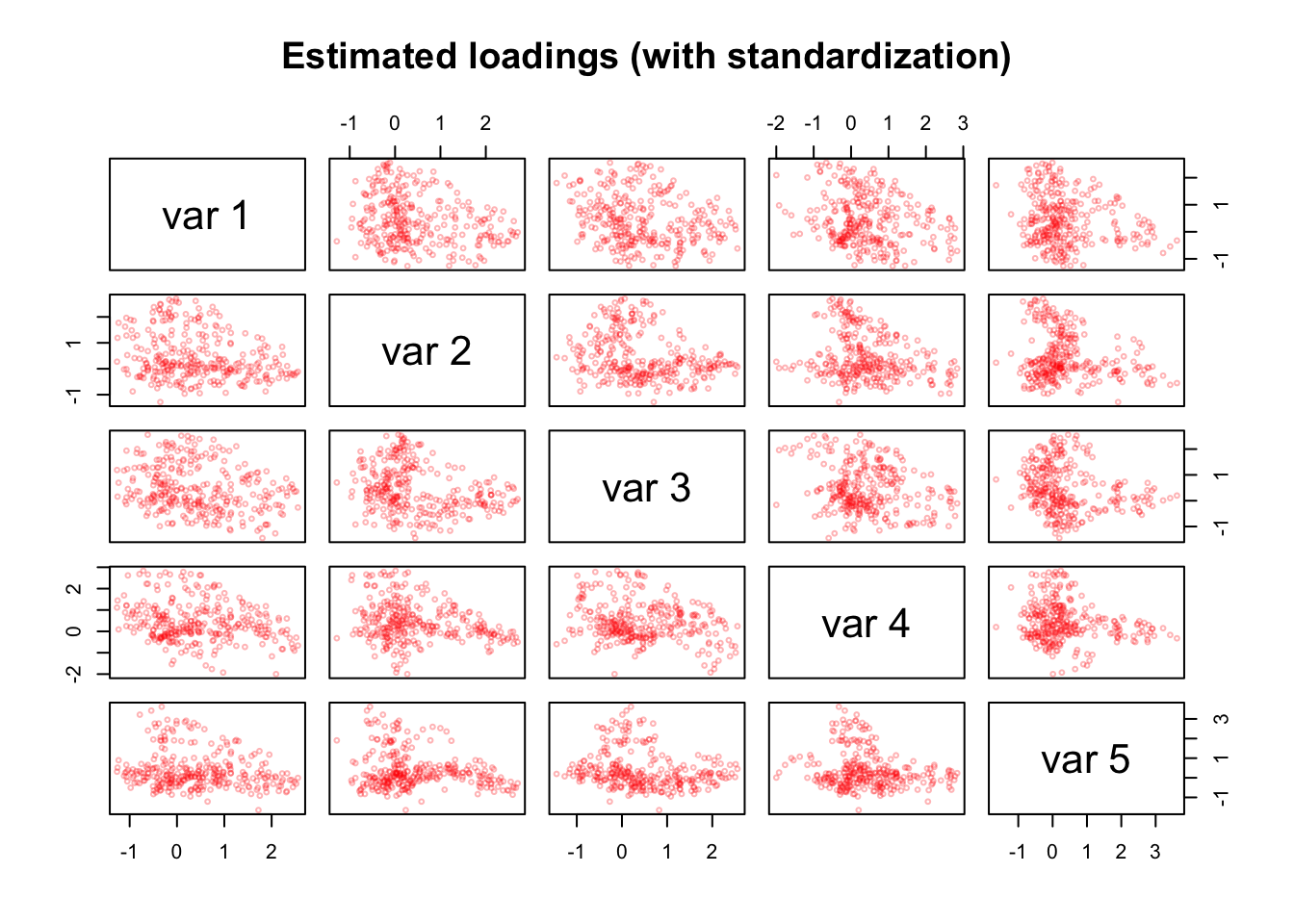
However, we find noisy streaks in the estimated loading matrix \(\hat{Y}\). This simple structure is in line with the construction process of the personality questionnaire, which has the goal that each item measures only a single Big Five factor. Streaks are even more pronounced when extracting 30 components.
Finally, we interpret the components by highlighting the 10 items with the highest absolute loadings on each component.
In [8]:
n = 10
top_vars_items_z = data.frame(
  Extraversion = names(sort(abs(pca_items_z$Y[, 1]), decreasing = TRUE)[1:n]),
  Conscientiousness = names(sort(abs(pca_items_z$Y[, 2]), decreasing = TRUE)[1:n]),
  Agreeableness = names(sort(abs(pca_items_z$Y[, 3]), decreasing = TRUE)[1:n]),
  EmotionalStability = names(sort(abs(pca_items_z$Y[, 4]), decreasing = TRUE)[1:n]),
  Openness = names(sort(abs(pca_items_z$Y[, 5]), decreasing = TRUE)[1:n])
)
kable(top_vars_items_z)| Extraversion | Conscientiousness | Agreeableness | EmotionalStability | Openness |
|---|---|---|---|---|
| E1.1 | C6.8 | A6.8 | ES6.10 | O2.6 |
| E4.3 | C2.5 | O3.3 | ES1.3 | O2.5 |
| E2.7 | C4.9 | A6.10 | ES2.3 | O6.2 |
| E2.2 | ES5.6 | A6.2 | ES2.9 | O2.10 |
| E2.4 | C3.6 | O3.7 | ES2.7 | O5.4 |
| E2.8 | C5.6 | E1.7 | ES2.1 | O1.6 |
| E4.5 | C3.1 | A6.6 | ES2.8 | O1.2 |
| ES4.10 | C2.7 | A6.4 | ES3.7 | O1.9 |
| E2.6 | C4.5 | A6.5 | ES1.4 | O2.8 |
| E3.2 | C2.3 | O3.1 | ES2.6 | O2.1 |
With few exceptions, the item labels indicate that the implied Big Five personality factors (Extraversion, Conscientiousness, Agreeableness, Emotional Stability, Openness) were recovered as expected.
Mobile Sensing Data
In [9]:
phonedata_sensing = readRDS(file = "datasets/clusterdata.RDS")
phonedata_sensing = phonedata_sensing[, c(1:1821)]
The smartphone sensing data contains 1821 preprocessed variables. Of these variables, 772 contain missing values and not a single person has complete data on all variables. Thus, imputation of missing values seems a necessity when working with these data. We use very simple mean imputation here which is sufficient for the goal of our demonstration.
In [10]:
phonedata_sensing_imp = phonedata_sensing
for(col in colnames(phonedata_sensing_imp)) {
  phonedata_sensing_imp[which(is.na(phonedata_sensing_imp[[col]])), col] <-
    mean(phonedata_sensing_imp[[col]], na.rm = TRUE)
}
However, our results are quite similar for more elaborate imputation schemes. For the interested reader, we prepared data imputed with the miceRanger package in the sensitivity analysis document.
If you want to use that data, you have to set eval: true or manually run the following chunk in the .qmd file.
In [11]:
library(miceRanger)
mice_obj_sensing = readRDS(file = "mice_obj_sensing.RDS")
phonedata_sensing_imp = as.data.frame(completeData(mice_obj_sensing)[[1]])
Analysis with Standardization
In contrast to the item response data, there is a huge difference in the standard deviations of the smartphone sensing variables.
In [12]:
round(quantile(sapply(phonedata_sensing_imp, sd)), 2) 0% 25% 50% 75% 100%
0.02 0.21 2.13 12.81 1723949.43 Thus, it is important to standardize the variables before further analysis.
In [13]:
sensing_mat_imp_z = as.matrix(scale(phonedata_sensing_imp))
colnames(sensing_mat_imp_z) = colnames(phonedata_sensing_imp)
sensing_mat_imp_z = as(sensing_mat_imp_z, "dgCMatrix")
screeplot(vsp(sensing_mat_imp_z, rank = 50,
  degree_normalize = FALSE, center = TRUE))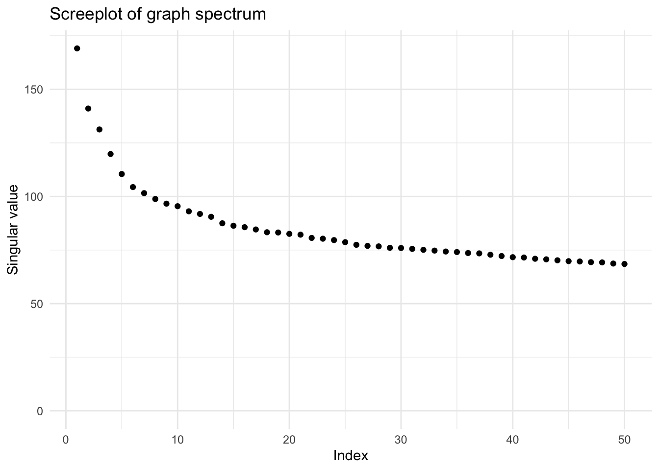
The screeplot does not show a clear gap or elbow for the smartphone sensing data. To keep it simple, we extract only 5 components here, but higher numbers also provide meaningful insights.
Again, we do not use degree normalization but we set center = TRUE despite standardizing the columns because row means also differ to some extent.
In [14]:
pca_sensing_imp_z = vsp(sensing_mat_imp_z, rank = 5,
  degree_normalize = FALSE, center = TRUE)
We search for radial streaks in the estimated component and loading matrices:
In [15]:
pairs(as.matrix(pca_sensing_imp_z$Z[, 1:5]), cex = 0.3, col = alpha("red", alpha = 0.1),
  main = "Estimated components (with standardization)")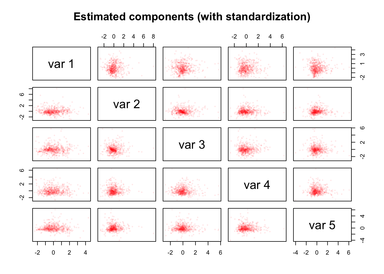
We do not find a clear indication of streaks in the estimated component matrix \(\hat{Z}\).
In [16]:
pairs(as.matrix(pca_sensing_imp_z$Y[, 1:5]), cex = 0.3, col = alpha("red", alpha = 0.1),
  main = "Estimated loadings (with standardization)")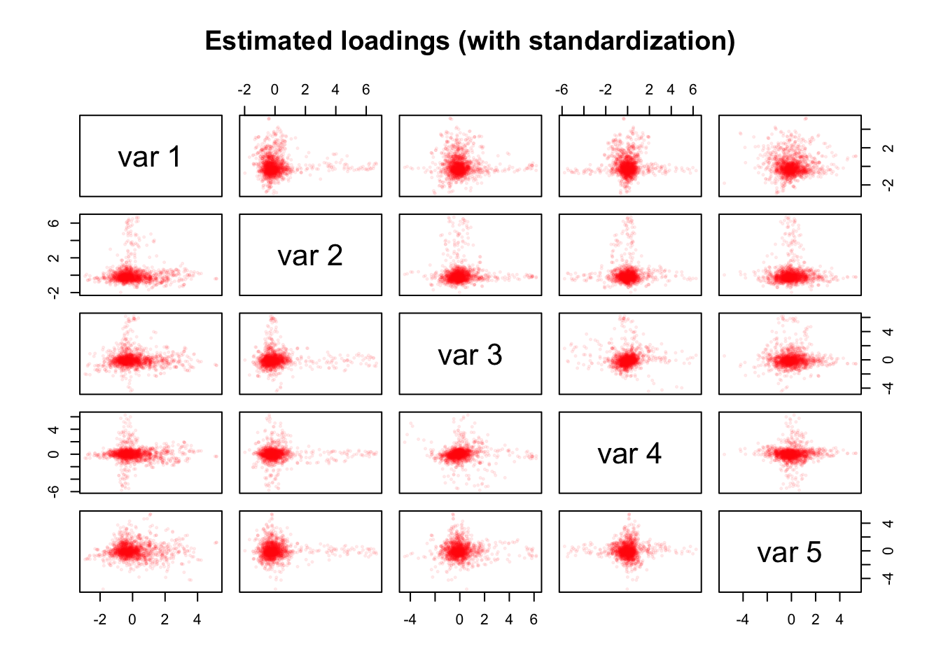
However, we find streaks in the estimated loading matrix \(\hat{Y}\). In contrast to the items of the personality questionnaire that have been constructed with simple structure in mind, no simple structure was implied when constructing the smartphone sensing variables. Nonetheless, the streaks would suggest that the smartphone sensing variables can be meaningfully clustered in this dataset.
For interpretation, we again highlight the 10 variables with the highest absolute loadings on each component.
In [17]:
n = 10
top_vars_z = data.frame(
  Apps_Usage = names(sort(abs(pca_sensing_imp_z$Y[, 1]), decreasing = TRUE)[1:n]),
  Calls = names(sort(abs(pca_sensing_imp_z$Y[, 2]), decreasing = TRUE)[1:n]),
  Music_Songs = names(sort(abs(pca_sensing_imp_z$Y[, 3]), decreasing = TRUE)[1:n]),
  Music_Audio_Features = names(sort(abs(pca_sensing_imp_z$Y[, 4]), decreasing = TRUE)[1:n]),
  Terrain = names(sort(abs(pca_sensing_imp_z$Y[, 5]), decreasing = TRUE)[1:n])
)
kable(top_vars_z)| Apps_Usage | Calls | Music_Songs | Music_Audio_Features | Terrain |
|---|---|---|---|---|
| daily_mean_num_unique_apps_week | daily_mean_num_cont_call | daily_mean_num_song | mean_music_loudness | daily_mean_neg_elev_change |
| daily_mean_num_unique_apps | daily_mean_num_cont | daily_mean_duration_music | mean_music_loudness_weekday | daily_mean_elev_change |
| daily_mean_num_unique_apps_weekend | daily_mean_num_cont_week | daily_max_num_uniq_song | sd_music_loudness | daily_mean_pos_elev_change |
| daily_mean_num_unique_Camera | daily_mean_num_cont_call_out | daily_mean_num_song_weekdays | mean_music_energy | daily_mean_elev_change_weekdays |
| daily_mean_num_unique_Camera_week | daily_sd_num_call_in | daily_mean_num_uniq_song | mean_music_loudness_weekend | daily_mean_elev_change_weekend |
| daily_mean_num_unique_Camera_weekend | IVI_calls | num_uniq_songs | mean_music_acousticness | daily_sd_elev_change |
| daily_mean_sum_events_daytime | daily_mean_num_cont_call_miss | daily_sd_num_song | mean_music_energy_weekday | daily_mean_num_.com.sonyericsson.home |
| daily_mean_sum_events_night | daily_mean_num_cont_weekend | num_songs | mean_music_acousticness_weekday | daily_mean_num_.com.sec.android.app.launcher |
| daily_mean_num_unique_Gallery | daily_mean_num_call_out | daily_mean_num_uniq_alb | sd_music_acousticness | daily_mean_num_.com.sec.android.gallery3d |
| daily_mean_num_unique_Gallery_week | daily_mean_num_cont_call_in | daily_sd_duration_music | mean_music_energy_weekend | daily_mean_num_.com.sonyericsson.album |
To summarize, with careful preprocessing and appropriate data standardization, PCA+VR seems to meaningfully cluster the smartphone sensing variables, as indicated by radial streaks in the estimated loading matrix \(\hat{Y}\). However, we did not find streaks in the estimated component matrix \(\hat{Z}\) so we cannot necessarily have high confidence that PCA+VR was able to estimate well identified person scores on these components.
The following cautionary example showcases what can happen when the smartphone sensing data is not preprocessed with enough care.
A Cautionary example: Analysis without Standardization
To simulate mindless data analysis, we do not standardize the smartphone sensing variables and use the default degree_normalize = TRUE in the vsp call, although this should not be a meaningful setting because we do not analyze binary network data here.
In [18]:
sensing_mat_imp = as.matrix(phonedata_sensing_imp)
colnames(sensing_mat_imp) = colnames(phonedata_sensing_imp)
sensing_mat_imp = as(sensing_mat_imp, "dgCMatrix")
screeplot(vsp(sensing_mat_imp, rank = 50,
  degree_normalize = TRUE, center = TRUE))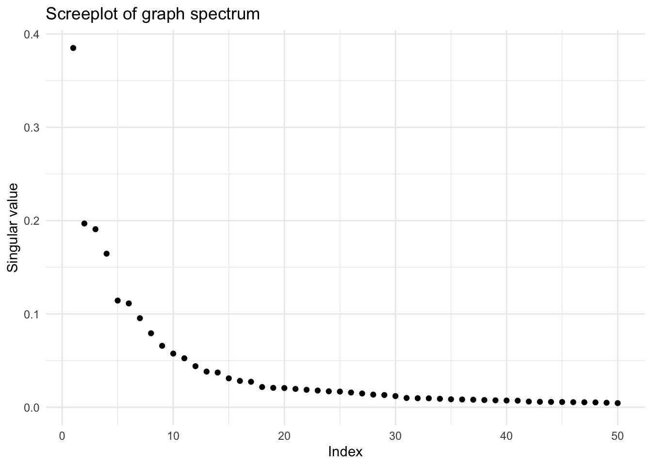
With these settings, the screeplot shows substantial gaps (in contrast to the previous analysis with standardization). To keep it simple, we decided to extract 5 components here, but the main insights from this exercise do not seem to depend on this number.
When searching for radial streaks in the estimated component and loading matrices, we notice interesting changes compared to the analysis with standardized variables
In [19]:
pca_sensing_imp = vsp(sensing_mat_imp, rank = 5,
  degree_normalize = TRUE, center = TRUE)
pairs(as.matrix(pca_sensing_imp$Z[, 1:5]), cex = 0.5, col = alpha("red", alpha = 0.2),
  main = "Estimated components (no standardization)")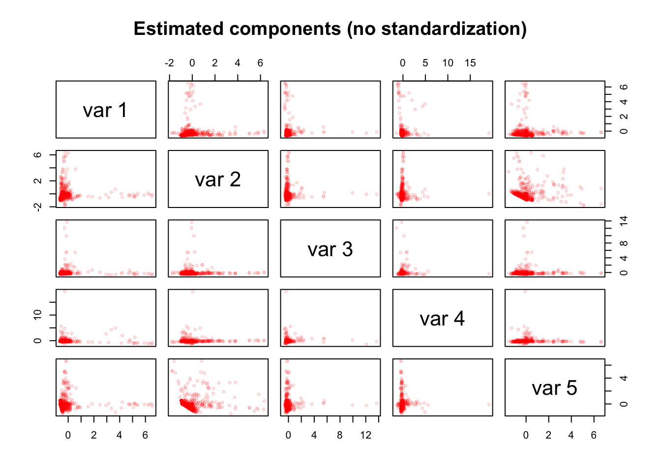
With these settings, we do find beautiful streaks in the estimated component matrix \(\hat{Z}\).
In [20]:
pairs(as.matrix(pca_sensing_imp$Y[, 1:5]), cex = 0.5, col = alpha("red", alpha = 0.4),
  main = "Estimated loadings (no standardization)")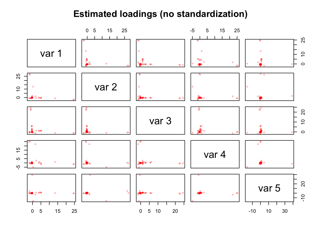
In contrast, streaks in the estimated loading matrix \(\hat{Y}\) are very extreme. To a careful analyst, this might perhaps raise some alarms that something might be wrong here…
In [21]:
n = 20
top_vars = data.frame(
  GPS1 = names(sort(abs(pca_sensing_imp$Y[, 1]), decreasing = TRUE)[1:n]),
  GPS2 = names(sort(abs(pca_sensing_imp$Y[, 2]), decreasing = TRUE)[1:n]),
  GPS3 = names(sort(abs(pca_sensing_imp$Y[, 3]), decreasing = TRUE)[1:n]),
  GPS4 = names(sort(abs(pca_sensing_imp$Y[, 4]), decreasing = TRUE)[1:n]),
  GPS5 = names(sort(abs(pca_sensing_imp$Y[, 5]), decreasing = TRUE)[1:n])
)
red_vars = unique(unlist(top_vars))
kable(top_vars)| GPS1 | GPS2 | GPS3 | GPS4 | GPS5 |
|---|---|---|---|---|
| maxDistance | huberM_time_spent_home | huberM_distance_covered_weekend | huberM_daily_max_dist_home | huberM_time_spent_home_weekend |
| max_distance_home | huberM_time_spent_home_weekday | huberM_distance_covered_daily | huberM_daily_max_dist_home_weekday | durationHome |
| rog | durationHome | huberM_distance_covered_weekday | huberM_daily_max_dist_home_weekend | huberM_time_spent_home_weekday |
| SDD | max_distance_home | huberM_max_dist_two_points_weekend | durationHome | huberM_daily_max_dist_home_weekend |
| SDD_daytime | maxDistance | huberM_max_dist_two_points_daily | SDD_nighttime | SDD_weekend |
| SDD_weekend | huberM_time_spent_home_weekend | huberM_max_dist_two_points_weekday | max_distance_home | SDD_sat |
| SDD_sat | huberM_daily_max_dist_home_weekend | huberM_rog_weekends | maxDistance | SDD_nighttime |
| SDD_weekday | huberM_daily_time_spent_home | huberM_rog_daily | SDD | SDD |
| SDD_nighttime | huberM_daily_max_dist_home | huberM_rog_weekdays | rog | mean_dur_wakeLeaveHome_weekend |
| huberM_daily_max_dist_home_weekday | rog | Qn_rog_weekends | SDD_sat | huberM_distance_covered_daily |
| huberM_time_spent_home_weekday | huberM_distance_covered_daily | huberM_rog_nightly | huberM_max_dist_two_points_weekend | mean_time_firstLeave |
| huberM_daily_max_dist_home_weekend | huberM_daily_max_dist_home_weekday | max_distance_home | SDD_daytime | mean_time_LeaveHome_weekday |
| huberM_time_spent_home | SDD_nighttime | huberM_daily_max_dist_home_weekend | Qn_rog_weekends | huberM_rog_weekends |
| huberM_daily_max_dist_home | huberM_distance_covered_weekday | SDD | huberM_time_spent_home_weekend | SDD_daytime |
| huberM_distance_covered_weekend | huberM_distance_covered_weekend | SDD_daytime | huberM_daily_time_spent_home | huberM_distance_covered_weekday |
| huberM_distance_covered_weekday | huberM_max_dist_two_points_weekend | SDD_weekday | huberM_distance_covered_weekday | mean_dur_wakeLeave |
| huberM_distance_covered_daily | SDD_weekend | SDD_nighttime | huberM_distance_covered_daily | mean_time_lastHome |
| huberM_max_dist_two_points_daily | huberM_rog_weekends | SDD_weekend | huberM_rog_weekends | huberM_rog_nightly |
| huberM_max_dist_two_points_weekend | mean_time_lastHome | maxDistance | huberM_max_dist_two_points_daily | mean_time_LeaveHome |
| huberM_max_dist_two_points_weekday | daily_sd_elev_change | SDD_sat | huberM_max_dist_two_points_weekday | mean_time_lastHome_weekend |
Indeed, when looking at the top variables with the highest absolute loadings on each component, they do not seem to have a simple structure and are hard to interpret.
In fact, the top 20 variables loading on all components include only 36 unique variables.
Most of these variables seem to be based on GPS data in some way.
All of these variables have extremely high standard deviations.
In [22]:
sapply(phonedata_sensing_imp[, red_vars], sd) maxDistance max_distance_home
1723949.4317 1658119.0296
rog SDD
593713.5051 104176.6763
SDD_daytime SDD_weekend
110929.5007 127175.3902
SDD_sat SDD_weekday
118107.2267 96185.8329
SDD_nighttime huberM_daily_max_dist_home_weekday
89259.8191 386481.1616
huberM_time_spent_home_weekday huberM_daily_max_dist_home_weekend
396556.4282 597855.8383
huberM_time_spent_home huberM_daily_max_dist_home
362331.9954 395986.1722
huberM_distance_covered_weekend huberM_distance_covered_weekday
273597.0960 236849.2267
huberM_distance_covered_daily huberM_max_dist_two_points_daily
228491.3102 36548.9043
huberM_max_dist_two_points_weekend huberM_max_dist_two_points_weekday
51418.1852 37995.9337
durationHome huberM_time_spent_home_weekend
630997.9841 356598.2761
huberM_daily_time_spent_home huberM_rog_weekends
23839.3676 19736.6958
mean_time_lastHome daily_sd_elev_change
13992.7979 652.7301
huberM_rog_daily huberM_rog_weekdays
13893.6231 15196.8947
Qn_rog_weekends huberM_rog_nightly
21541.5438 15109.0978
mean_dur_wakeLeaveHome_weekend mean_time_firstLeave
13712.9354 12298.1192
mean_time_LeaveHome_weekday mean_dur_wakeLeave
12196.0186 12383.4894
mean_time_LeaveHome mean_time_lastHome_weekend
12203.8207 14425.9489 In addition, all of these variables contain missing values in the original dataset and the number of missings is quite high for some of them.
In [23]:
sapply(phonedata_sensing[, red_vars], function(x) sum(is.na(x))) maxDistance max_distance_home
58 69
rog SDD
63 60
SDD_daytime SDD_weekend
66 107
SDD_sat SDD_weekday
114 82
SDD_nighttime huberM_daily_max_dist_home_weekday
110 91
huberM_time_spent_home_weekday huberM_daily_max_dist_home_weekend
97 204
huberM_time_spent_home huberM_daily_max_dist_home
69 69
huberM_distance_covered_weekend huberM_distance_covered_weekday
120 83
huberM_distance_covered_daily huberM_max_dist_two_points_daily
67 60
huberM_max_dist_two_points_weekend huberM_max_dist_two_points_weekday
110 77
durationHome huberM_time_spent_home_weekend
69 189
huberM_daily_time_spent_home huberM_rog_weekends
69 133
mean_time_lastHome daily_sd_elev_change
70 5
huberM_rog_daily huberM_rog_weekdays
74 90
Qn_rog_weekends huberM_rog_nightly
133 132
mean_dur_wakeLeaveHome_weekend mean_time_firstLeave
5 60
mean_time_LeaveHome_weekday mean_dur_wakeLeave
123 5
mean_time_LeaveHome mean_time_lastHome_weekend
93 230 Our suspicion is that the radial streaks in the estimated component matrix \(\hat{Z}\) might be a result of these GPS variables, which dominate the solution from PCA+VR without standardization but are hidden behind the remaining variables when standardization is used.
To confirm some of these suspicions, we repeat PCA+VR on only these 36 variables, but now use standardization again. This results in 2 strong components with pronounced but odd-looking and not perfectly aligned streaks in both \(\hat{Z}\) and \(\hat{Y}\).
In [24]:
sensing_mat_imp_z_red = as.matrix(scale(phonedata_sensing_imp[, red_vars]))
colnames(sensing_mat_imp_z_red) = colnames(phonedata_sensing_imp[, red_vars])
sensing_mat_imp_z_red = as(sensing_mat_imp_z_red, "dgCMatrix")
screeplot(vsp(sensing_mat_imp_z_red, rank = 20,
  degree_normalize = FALSE, center = TRUE))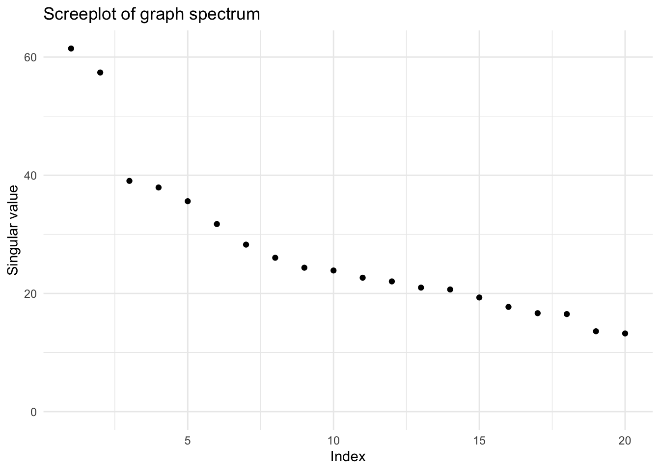
In [25]:
pca_sensing_imp_z_red = vsp(sensing_mat_imp_z_red, rank = 2,
  degree_normalize = FALSE, center = TRUE)
pairs(as.matrix(pca_sensing_imp_z_red$Z[, 1:2]), cex = 0.5, col = alpha("red", alpha = 0.2),
  main = "Estimated components (reduced itemset with standardization)")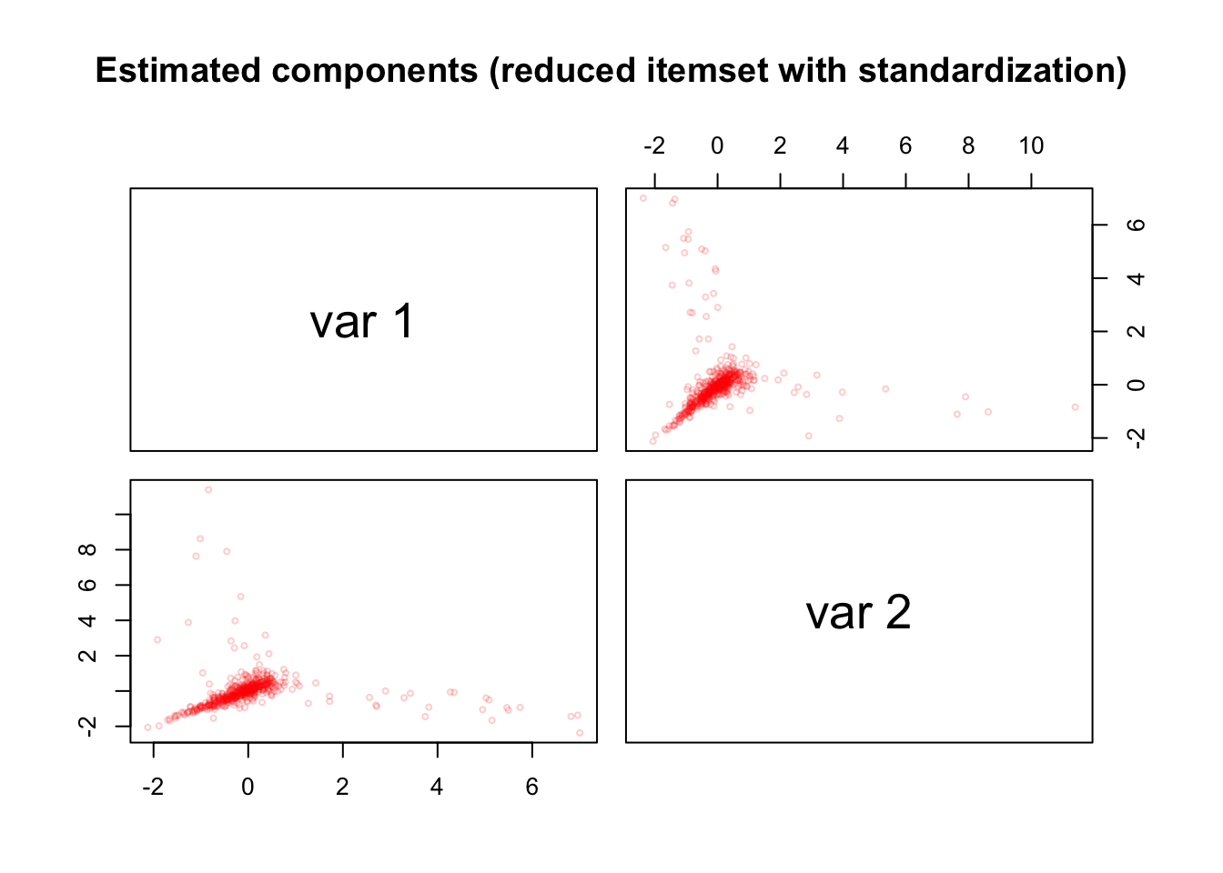
In [26]:
pairs(as.matrix(pca_sensing_imp_z_red$Y[, 1:2]), cex = 0.5, col = alpha("red", alpha = 0.6),
  main = "Estimated loadings (reduced itemset with standardization)")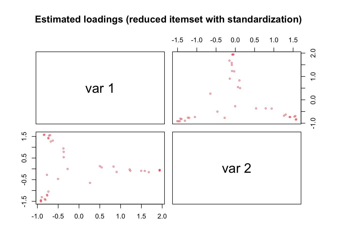
In [27]:
n = 10
top_vars = data.frame(
  GPS1 = names(sort(abs(pca_sensing_imp_z_red$Y[, 1]), decreasing = TRUE)[1:n]),
  GPS2 = names(sort(abs(pca_sensing_imp_z_red$Y[, 2]), decreasing = TRUE)[1:n])
)
kable(top_vars)| GPS1 | GPS2 |
|---|---|
| rog | mean_time_LeaveHome |
| maxDistance | mean_time_LeaveHome_weekday |
| max_distance_home | mean_time_firstLeave |
| SDD | mean_dur_wakeLeave |
| SDD_daytime | huberM_max_dist_two_points_daily |
| SDD_weekend | huberM_rog_daily |
| SDD_sat | huberM_max_dist_two_points_weekday |
| SDD_weekday | huberM_distance_covered_daily |
| huberM_rog_daily | huberM_time_spent_home_weekday |
| huberM_max_dist_two_points_weekday | huberM_time_spent_home |
Simulation: Correlated Factors
Another important aspect of psychological applications of PCA+VR are correlated factors (e.g., the personality dimensions conscientiousness and neuroticism are thought to correlate around \(-0.4\); Linden et al. (2010)), thus oblique rotations are often argued for. Interestingly, R&Z show as a side result that the results of PCA+VR can be used to also estimate correlated factors in situations which are relevant for psychological measurement models.
In [28]:
library(vsp)
library(Matrix)
library(scales)
library(mvtnorm)
Here we demonstrate that \(\hat{Z}\hat{B}\) (up to a change of units) estimates correlated factors simulated from a leptokurtic distribution:
- Simulate correlated factor scores from a multivariate leptokurtic distribution.
In [29]:
set.seed(3)

n = 10000
rho = 0.7
# adapted from https://github.com/RoheLab/vsp-paper/blob/master/scripts/makeFigure1.R
Z_star = scale(matrix(sample(c(-1,1), 2 * n, T) *
    rexp(n * 2, rate = 2) ^ 1.3, ncol = 2))
cor_mat = matrix(c(1, rho, rho, 1), ncol = 2)
Z = Z_star %*% chol(cor_mat)
We first simulate two-dimensional uncorrelated standardized scores from a leptokurtic distribution (\(Z^*\)). Correlated scores (\(Z\)) are then constructed by multiplying the uncorrelated scores with the Cholesky factor of a correlation matrix with the desired correlation (\(\rho = 0.7\)).
In [30]:
pairs(Z, cex = 0.5, col = alpha("red", alpha = 0.2),
  main = "True correlated factors")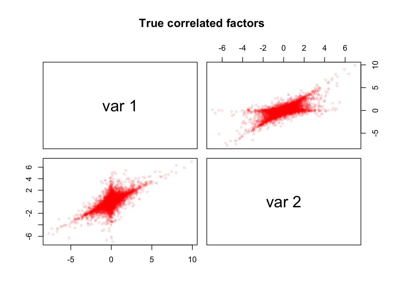
When plotting the simulated component scores in the \(Z\) matrix, we see non-orthogonal streaks (i.e. oblique components).
- Simulate item response data.
In [31]:
k = 2
vpf = 20
d = vpf*k

pf_low = 0.8
pf_upper = 0.95
sf_low = 0
sf_upper = 0

loadings = function(k, d, vpf, pf_low, pf_upper, sf_low, sf_upper){
  x = runif(d, pf_low, pf_upper)
  y = runif(d*(k-1) , sf_low, sf_upper)
  i = 1:(d)
  j = rep(1:k, each = vpf)
  L = matrix(NA, d, k)
  L[cbind(i, j)] = x
  L[is.na(L)] = y
  L
}

Y = loadings(k, d, vpf, pf_low, pf_upper, sf_low, sf_upper)
A =  Z %*% t(Y) + rnorm(n * d, sd = 0.1)
We create a loading matrix \(Y\) with simple structure and simulate the data matrix \(A\) with \(ZY^T\) and add some normally distributed noise.
- Perform PCA + Varimax
In [32]:
pca_sim = vsp(A, rank = 2, degree_normalize = FALSE)- Estimate uncorrelated component scores \(Z\)
In [33]:
pairs(as.matrix(pca_sim$Z[, 1:2]), cex = 0.5, col = alpha("red", alpha = 0.2),
  main = "Estimated uncorrelated factors")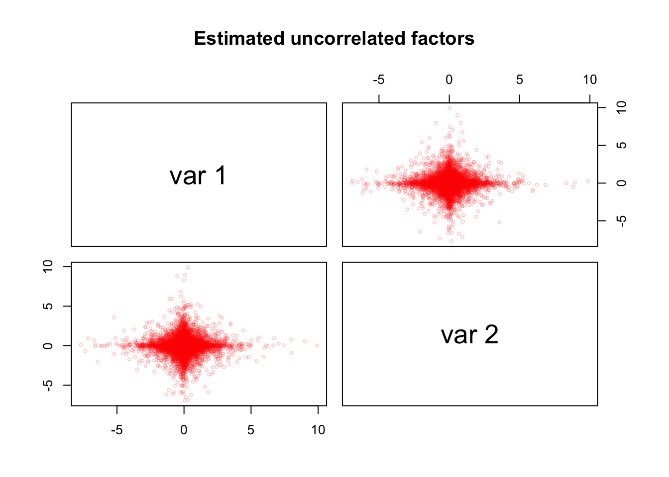
When plotting the \(\hat{Z}\) matrix returned from PCA+VR, we see orthogonal streaks similar to \(Z^*\).
- Estimate correlated component scores \(Z\)
In [34]:
ZB_hat = as.matrix(pca_sim$Z) %*% as.matrix(pca_sim$B)
pairs(ZB_hat, cex = 0.5, col = alpha("red", alpha = 0.2),
  main = "Estimated correlated factors")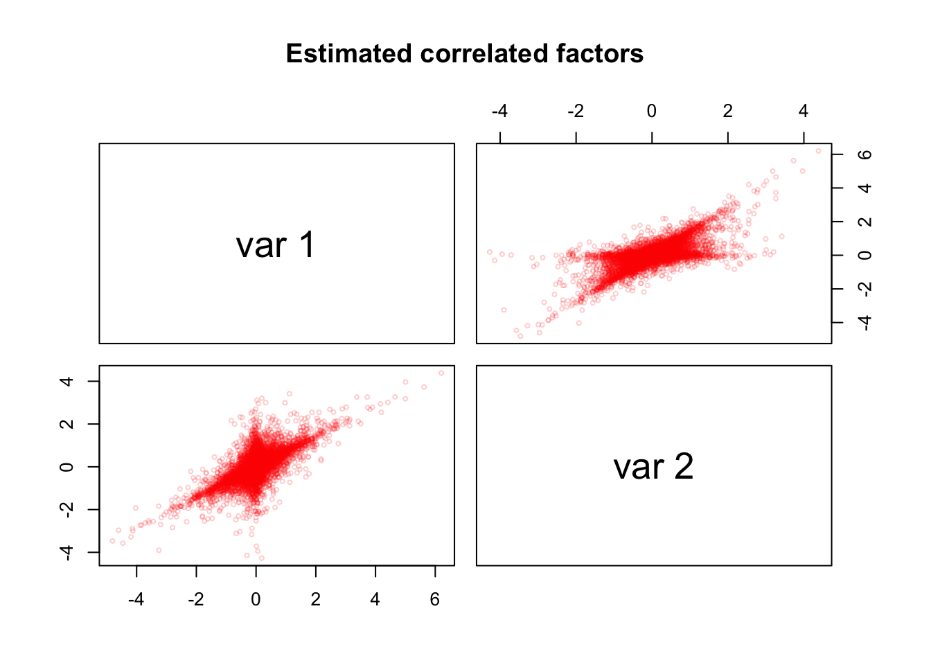
However, the matrix \(\hat{Z}\hat{B}\) contains correlated components similar to \(Z\).
- Estimate correlation between components
In [35]:
cor(ZB_hat) [,1] [,2]
[1,] 1.0000000 0.7033317
[2,] 0.7033317 1.0000000We can verify that the correlation of the scores in \(\hat{Z}\hat{B}\) are close to the true correlation in \(Z\) (\(\rho = 0.7\)).
Our simulation seems to demonstrate the results from sections 7.1 and 7.2 in R&Z, which state that if scores in \(Z\) are correlated; scores in \(Y\) are centered, independent, and leptokurtic; and the true \(B\) is proportional to the identity matrix, then the \(\hat{B}\) matrix returned from PCA+VR estimates the Cholesky factor of the covariance matrix \(Z^TZ\) (up to a change of unit). Note that because our scores in \(Z\) were scaled, \(Z^TZ\) is equal to the correlation matrix in our demonstration.
Open Questions
Surprisingly, the exact scores in \(Z\) (in the same unit) seem to be estimated by \(\hat{Z}\hat{B}\cdot d^{1/8}\).
In [36]:
nrows = 10
compare_scores = data.frame(
  z1 = Z[1:nrows, 1],
  z1_hat = ZB_hat[1:nrows, 1] * d^(1/8),
  z2 = Z[1:nrows, 2],
  z2_hat = ZB_hat[1:nrows, 2] * d^(1/8),
row.names = NULL)
kable(compare_scores)| z1 | z1_hat | z2 | z2_hat |
|---|---|---|---|
| -0.8175379 | -0.8258829 | 0.3337107 | 0.3052195 |
| 0.1451648 | 0.1404835 | 0.9071543 | 0.9425134 |
| 0.3726275 | 0.3342478 | -0.0673917 | -0.0741674 |
| -0.0312845 | -0.0496686 | 1.0465835 | 1.0630476 |
| 0.0533857 | 0.0278354 | -0.0289375 | -0.0004230 |
| 2.7693088 | 2.7368688 | 2.0474298 | 2.0732120 |
| 0.6403584 | 0.6849868 | 0.3958977 | 0.3967702 |
| -0.5940332 | -0.5576306 | -0.1732053 | -0.1453989 |
| -0.2614659 | -0.2740095 | -0.7323451 | -0.7558590 |
| 0.6697399 | 0.6585350 | 0.4020305 | 0.4119104 |
Unfortunately, we were not able not determine why or whether this might be just a coincidence here. To conclude, we agree with the following comment in R&Z (Rohe & Zeng, 2023) and are looking forward to further research in this direction:
Taken together, this all suggests that the B matrix provides a path to understanding “correlation among the factors.” Understanding this phenomenon is an active area of research in our lab.
References
Arendasy, M., Sommer, M., & Feldhammer, M. (2011). Manual Big-Five Structure Inventory BFSI. Schuhfried Gmbh, Mödling.
Linden, D. van der, Nijenhuis, J. te, & Bakker, A. B. (2010). The General Factor of Personality: A meta-analysis of Big Five intercorrelations and a criterion-related validity study. Journal of Research in Personality, 44(3), 315–327. https://doi.org/10.1016/j.jrp.2010.03.003
Pargent, F., Goretzko, D., & Oertzen, T. von. (2023). Florian Pargent, David Goretzko and Timo von Oertzen’s contribution to the Discussion of “Vintage Factor Analysis with Varimax Performs Statistical Inference” by Rohe
& Zeng. Journal of the Royal Statistical Society Series B: Statistical Methodology, 85(4), 1087–1088. https://doi.org/10.1093/jrsssb/qkad054
& Zeng. Journal of the Royal Statistical Society Series B: Statistical Methodology, 85(4), 1087–1088. https://doi.org/10.1093/jrsssb/qkad054
Rohe, K., & Zeng, M. (2023). Vintage factor analysis with Varimax performs statistical inference. Journal of the Royal Statistical Society Series B: Statistical Methodology, 85(4), 1037–1060. https://doi.org/10.1093/jrsssb/qkad029
Stachl, C., Au, Q., Schoedel, R., Gosling, S. D., Harari, G. M., Buschek, D., Völkel, S. T., Schuwerk, T., Oldemeier, M., Ullmann, T., Hussmann, H., Bischl, B., & Bühner, M. (2020). Predicting personality from patterns of behavior collected with smartphones. Proceedings of the National Academy of Sciences of the United States of America, 117(30), 17680–17687. https://doi.org/10.1073/pnas.1920484117