---
title: "Perturbative Techniques"
aliases: [2_ANONYMISATION_TECHNIQUES/2_4_Perturbative.html]
bibliography: ../references.bib
execute:
cache: true
---
::: {.callout-tip collapse="true"}
## Learning Objective
- Apply selected **perturbative techniques** in R.
:::
```{r setup}
#| include: false
# Setup: load packages, data, and the saved sdcObject
library(sdcMicro)
library(tidyverse)
set.seed(1) # only so the numbers in this tutorial stay the same on every render; delete for a real application
data_withoutidentifiers <- read.csv(here::here("simulated-data-noidentifiers.csv")) # Change based on the location of your data file
sdc_nonpert <- readRDS(here::here("sdc-nonpert.rds")) # Change based on the location of your Sdc-object file
```
The core idea behind perturbative techniques is to introduce **controlled changes to data values**. Unlike non-perturbative techniques that hide or remove information, perturbative methods keep all records and variables in the dataset but **alter the values themselves**. The key requirement is that the changes should be large enough to prevent re-identification but small enough that the overall statistical properties of the data (means, variances, correlations) are preserved.
In most cases, perturbation does not increase k-anonymity, since values are not generalized but instead just changed. Recall that k-anonymity counts how many records share the same combination of indirect identifiers. It only goes up when distinct values are collapsed into shared, broader categories, the way recoding or suppression does. Perturbation works differently: it swaps each value for another *specific* value rather than a broader category, so a record that was unique on its indirect identifiers stays unique, the only difference is that its values change. It may reshuffle which records look unusual, but it does not merge them into the larger shared groups that a higher k requires.
On top of that, we typically perturb continuous variables such as income, which are not even part of the categorical key that k-anonymity is calculated on in the first place. Perturbation therefore adds another layer of protection—especially for continuous variables—rather than raising k-anonymity. Exceptions to this rule are microaggregation and rounding, which are perturbative, but also generalize data and therefore contribute to k-anonymity as well.
::: {.callout-note collapse="false"}
## Can I Just Delete the Variable Instead?
If the values you publish are not the real ones anymore, why keep the variable at all?
The answer is that deletion and perturbation remove **different things**. Deleting a variable removes the information for everyone and for every purpose. Perturbation removes only the **precision** of individual values, which is usually where the risk sits, and keeps the structure that is of interest for research.
Let's take `income` in our dataset as an example. What makes a data point identifiable is not that someone *has* an income—it is that one participant has exactly **€902,234.42**, more than seventeen times the sample median of about €52,000 and one of only three incomes above €110,000. Anyone who knows even vaguely that a particular participant is a top earner can easily point to that individual. But almost no reuse of these data depends on that exact amount:
- A colleague testing whether **income is related to political opinions** needs the association, not the individual values. After microaggregation or a modest amount of noise, the correlation and the regression coefficients stay close to those from the original data. With `income` deleted, this analysis is not possible at all.
- A researcher **pooling your data with other studies** needs a comparable income variable. A slightly noisy one still works; a missing one excludes your study from the pool.
`years_in_job` works the same way. The longest tenure in the sample is **32 years**, with the next-longest at 24—in a sample of 200, that makes a person very identifiable. But no plausible analysis needs "32" rather than "roughly 30, in the longest-tenure group." Deleting the variable would remove a legitimate predictor from every future analysis in order to protect a single record.
:::
In this chapter, I will present a few perturbative techniques introduced in @Carvalho2023_SurveyPrivacyPreservingTechniques.
## Examples of Perturbative Techniques
### Swapping
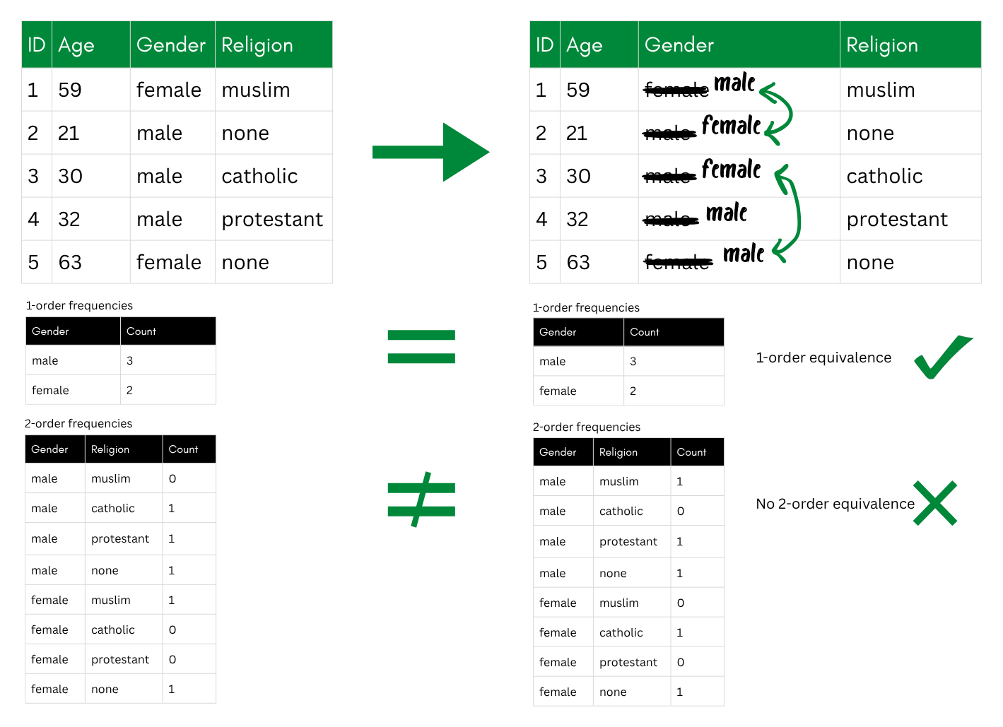
Swapping **exchanges values of a variable between participants**. Instead of altering the values themselves, it breaks the link between a record and the individual it belongs to.
There are two main variants. **Record swapping** (also known as data swapping) applies to categorical variables: values like gender or country of residence are swapped between records. A useful property here is t-order equivalence. For example, 1-order equivalence means the marginal frequencies are preserved (same number of males and females as before), and 2-order equivalence means joint frequencies are also preserved (same number of males and females from each country).
{fig-alt="A before-and-after table where gender values are swapped between records; frequency tables below show that 1-order frequencies stay equal while 2-order frequencies change."}
**Rank swapping** applies to continuous variables: values are only swapped with other values that are close in rank, which limits how much the distribution is distorted.
The main **advantage** of swapping is that it removes the relationship between a record and the individual without introducing new values that never existed in the data. It can protect rare and unique values and works across variable types. On the **downside**, non-random swapping requires careful implementation, and swapping can produce unusual combinations of values that did not exist in the original data.
### Re-Sampling
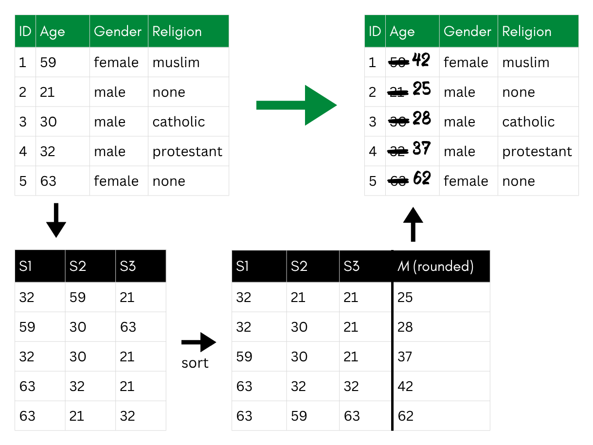
Re-sampling **replaces original values with averages** computed from bootstrap samples [@hundepool2026]. You draw multiple independent bootstrap samples from the original data with replacement, with the same sample size as your original data, and sort the values within each sample. You then compute the average of the smallest values across all samples, then of the second-smallest ones, and so forth, and replace the corresponding original values (i.e., the smallest original value with the average of the smallest values in the samples, etc.). The result preserves the overall distribution, but individual values no longer correspond to real observations.
{fig-alt="A before-and-after table where the exact ages are replaced with mean values of sub-samples."}
### Noise
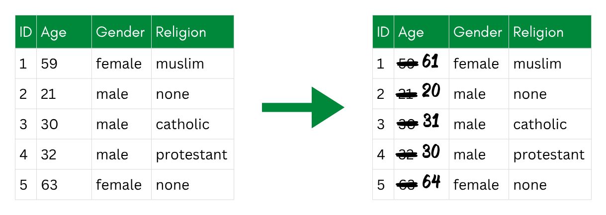
Noise addition (also known as randomization) **adds a random value** to each original value. The most common form is **additive noise**: a random draw from a distribution (typically normal with mean 0) is added to the original value. **Multiplicative noise** works similarly but multiplies the original value by a random factor, which scales the perturbation to the magnitude of the variable.
The noise can be uncorrelated—each value gets an independent random draw—or correlated with the original values, which better preserves the correlation structure between variables. Transformations of the variable (e.g., log-transforming income before adding noise) are also possible and can improve the result for skewed distributions.
{fig-alt="A before-and-after table where each age is replaced with a slightly different, noisy value."}
::: {.callout-note collapse="false"}
## Differential Privacy
**How much noise is enough?** In this tutorial, we look at this question empirically—add noise, then measure the remaining risk (as you will do in the exercise below). **Differential privacy** approaches the same question from another perspective: you set a privacy level first, and the noise is then calibrated mathematically so that a formal guarantee holds. This guarantee applies to an **algorithm**, **not to the dataset itself**: the algorithm's output must be essentially the same whether or not any single individual's data is included, so an attacker learns (almost) nothing about anyone's participation. However, this still achieves a certain privacy level for this one dataset.
You already know a technique that provides this guarantee: the [randomized response technique](../foundations/mechanisms.qmd#randomized-response-technique) from the chapter on mechanisms. Because each answer is randomized with known probabilities, a "yes" says nothing about any individual, yet the true prevalence can still be estimated.
That example also shows a practical difference from an approach like k-anonymity, which requires a trusted party holding the complete dataset to anonymize it. With differential privacy, noise can instead be added **locally**—in the case of randomized response, by each participant themselves, before their data is even collected.
**Helpful resources:**
- The R package [DPpack](https://cran.r-project.org/web/packages/DPpack/index.html) provides functions for applying differential privacy to common statistical analyses in R.
- For an accessible introduction to the concepts behind differential privacy, see this book [@dwork2014].
:::
### Microaggregation
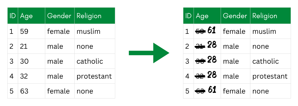
Microaggregation **groups records by similarity on the variable of interest and replaces each value with a group aggregate**—usually the mean or median. Records within the same group end up sharing the same value, which makes it impossible to single out an individual based on that variable alone.
{fig-alt="A before-and-after table where ages are replaced with group averages, with several records sharing the same value."}
The quality of the result depends on how homogeneous the groups are: the more similar the original values within a group, the less information is lost when replacing them with the group mean. This is why the grouping algorithm matters. The default in `sdcMicro`, `mdav` (Maximum Distance to Average Vector), tries to form compact groups to minimize distortion.
### Rounding
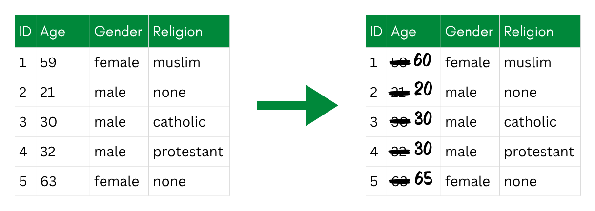
**Rounding replaces exact values with rounded versions**. For example, one can round income to the nearest €1,000, or age to the nearest 5 years. It is the simplest perturbative technique and is easy to explain and verify. The downside is that it provides relatively weak protection on its own, since the original value can often be guessed within a small range, or loses quite a lot of data in case of larger ranges that are rounded to the same value.
{fig-alt="A before-and-after table where ages are rounded to values such as 65, 20, and 30."}
### PRAM
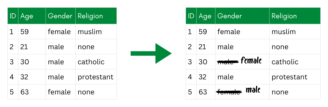
PRAM (Post RAndomization Method) applies to categorical variables. Each value is **randomly recoded to a different category with a certain probability** defined in a transition matrix. For example, a participant recorded as "male" might be recoded to "female" with probability 0.05 and kept as "male" with probability 0.95. The transition probabilities are chosen so that the distribution of the variable is approximately preserved, even though individual values may have changed.
{fig-alt="A before-and-after table where two of the gender values are randomly changed to a different category."}
This technique can be applied to the `keyVars` we defined in the `sdcObject` earlier, but does not improve k-anonymity indicators since it doesn't reduce the amount of unique combinations but rather changes the accuracy of those combinations. It is therefore an additional level of protection that `sdcMicro` indicators cannot measure.
## Keeping Utility
After applying any perturbative technique, you should compare key statistics (means, standard deviations, correlations, regression coefficients) between the original and perturbed datasets. If the differences are small enough for your purposes, the perturbation has preserved utility. I cover formal utility measures in [the chapter on balancing utility and privacy](../privacy-openness/balancing).
## Pro and Contra of Using Perturbative Techniques
Pros:
- No records or variables are removed; the dataset stays complete.
- Statistical properties like means, variances, and correlations can be largely preserved.
- Easy to tune the privacy-utility trade-off by adjusting the noise level or group size.
Cons:
- Individual values are no longer accurate. This makes perturbative techniques unsuitable if exact values matter—for example, if a researcher needs to verify that a specific participant had a specific income.
- Risk of reverse-engineering: if the perturbation method and its parameters are known, an attacker may be able to approximately reconstruct the original values.
- If applied too aggressively, perturbative techniques can distort subgroup statistics in ways that are hard to detect.
## Exercise: Applying Perturbative Techniques
Let's try out two common perturbative techniques: microaggregation and noise. Conveniently, both are available directly in `sdcMicro`.
Continue working with `sdc_nonpert` from the previous exercise.
1. **Apply microaggregation** (with the function `microaggregation()`) **to income** using the default method (`"mdav"`). Start with a group size of `aggr = 5`.
2. **Add additive noise to income** (with the function `addNoise()`) as an alternative. Start with a noise parameter of 1.
3. **Compare the methods:** Which parameters do you need to achieve similar levels of protection?
::: {.callout-tip collapse="false"}
## Work on Separate Copies
You cannot undo perturbation steps within the same `sdcObject`. Create a fresh copy of `sdc_nonpert` before trying the second method so you can compare them side-by-side.
:::
::: {.callout-important collapse="true"}
## Solution
#### Microaggregation
I start by applying microaggregation with a group size of 5 on a new `sdcObject`.
```{r}
# Microaggregation: replace income with group means (group size 5)
sdc_micro <- microaggregation(
  obj       = sdc_nonpert,
  variables = "income",
  aggr      =  5,         # group size
  method    = "mdav"      # Maximum Distance to Average Vector
)

sdc_micro
print(sdc_micro, type = "risk")
data_micro <- extractManipData(sdc_micro) # Extract the manipulated data
```
`mdav` groups records by their distance to the group centroid, then replaces each value with the group mean. With `aggr = 5`, at least 5 records share the same income value, so singling out an individual is harder.
As the output of the `sdcObject` shows, the disclosure risk is reduced from up to 100% in the beginning to a range going only up to 77.5%.
#### Additive Noise
```{r}
# Additive noise on income
sdc_noise <- addNoise(
  obj       = sdc_nonpert,
  variables = "income",
  noise     = 3.5          # noise level as percentage of SD
)

print(sdc_noise, type = "risk")
sdc_noise
```
`addNoise()` draws from a normal distribution with mean 0 and standard deviation = `noise * sd(income)` and adds it to each value. Every record gets a unique (slightly wrong) income. When `noise = 3.5`, we add up to 3.5% of income's standard deviation. In relation to the starting point, we achieve a disclosure risk between 0% and 75.5%.
Let's save these objects for now. We will later come back to inspect the utility of both methods in [the chapter on balancing utility and privacy](../privacy-openness/balancing).
```{r}
# Save the perturbed sdcObjects for the balancing chapter
saveRDS(sdc_micro, here::here("sdc-micro.rds"))
saveRDS(sdc_noise, here::here("sdc-noise.rds"))
```
:::
Make sure never to publish the seed when you apply such methods.
## References





